Deriving 4th order approximation of a 2nd order derivative using Taylor Table method

We have to derive the following 4th order approximations of the second-order derivative.

1. Central difference

2. Skewed right-sided difference

3. Skewed left-sided difference

CENTRAL DIFFERENCING SCHEME

The number of nodes=p+q-1

where p is derivative.

q is the order of approximations

The no of nodes=2+4-1=5

DERIVATION:

To derive a fourth-order approximation for the second-order derivative

`(del^2u)/(delx^2)=(af(i-2)+bf(i-1)+cf(i)+df(i-1)+ef(i-1))/(dx^2)`

The Taylor table plays a role in easily expanding taylor series.

`dx^2f''(i)`	`f(i)`	`f'(i)dx`	`f''(i)dx^2`	`f'''(i)dx^3`	`f''''(i)dx^4`
`af(i-2)`	a	-2a	2a	-4a/3	2a/3
`bf(i-1)`	b	-b	b/2	-b/6	b/24
`cf(i)`	c	0	0	0	0
`df(i+1)`	d	d	d/2	d/6	d/24
`ef(i+2)`	e	2e	2e	4e/3	2e/3
sum of coefficients	0	0	1	0	0

This equation is solved using the matrix inversion method.

We have kept all coefficients 0 except `f''(i)dx^2` because that's the term we want to find(second-order derivative).

A.C=B

`[[1,1,1,1,1],[-2,-1,0,1,2],[2,1/2,0,1/2,2],[-4/3,-1/6,0,1/6,4/3],[2/3,1/24,0,1/24,2/3]].[[a],[b],[c],[d],[e]]=[[0],[0],[1],[0],[0]]`

C=inv(A).B

We get C as: a=-0.0833,b=1.3333,c=-2.5,d=1.3333,e=-0.0833

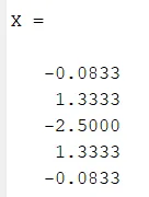
substituting in the equation we get

`(del^2u)/(delx^2)=(-0.0833f(i-2)+(1.3333)f(i-1)+(-2.5000)f(i)+(1.3333)f(i+1)+(-0.0833)f(i+2))/(dx^2)`

SKEWED RIGHT HAND DIFFERENCE SCHEME

No of nodes=p+q

Where, p is order of derivative.

q is order of approximations then,no of nodes=2+4=6.

Derivation:

`(del^2u)/(delx^2)=((af(i)+bf(i+2)+cf(i)+df(i+3)+ef(i+4))+(gf(i+5)))/(dx^2)`

expand the terms in this equation using taylor series expansion and represent in taylot table method.

`dx^2f''(i)`	`f(i)`	`f'(i)`	`f''(i)dx^2`	`f'''(i)dx^3`	`f''''(i)dx^4`	`f'''''(i)dx^5`
af(i)	a	0	0	0	0	0
bf(i+1)	b	b	`b/2`	`b/6`	`b/24`	`b/120`
cf(i+2)	c	2c	`(4c)/2`	`(8c)/6`	`(16c)/24`	`(32c)/120`
df(i+3)	d	3d	`(9d)/2`	`(27d)/6`	`(81d)/24`	`(243d)/120`
ef(i+4)	e	4e	`(16e)/2`	`(64e)/6`	`(256e)/24`	`(1024e)/120`
gf(i+5)	g	5g	`(25g)/2`	`(125g)/6`	`(625g)/24`	`(3125g)/120`
sum of co_efficient	0	0	1	0	0	0

A.X=B

`[[1,1,1,1,1,1],[0,1,2,3,4,5],[0,1/2,4/2,9/2,16/2,25/2],[0,1/6,8/6,27/6,64/6,125/6],[0,1/24,16/24,81/24,256/24,625/24],[0,1/120,32/120,243/120,1024/120,3125/120]].[[a],[b],[c],[d],[e],[g]]=[[0],[0],[1],[0],[0],[0]]`

X=inv(A)*B

we get X as: a=-3.7500, b=-12.8333, c=17.8333, d=-13.0000, e=5.0833, g=-0.8333

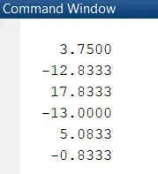
SKEWED LEFT HAND DIFFERENCE SCHEME

No of nodes=p+q

Where, p is order of derivative.

q is order of approximations then,no of nodes=2+4=6.

Derivation:

`(del^2u)/(delx^2)=((af(i-5)+bf(i-4)+cf(i-3)+df(i-2)+ef(i-1))+(gf(i)))/(dx^2)`

expand in terms of taylor table methods

`dx^2f''(i)`	`f(i)`	`f'(i)`	`f''(i)dx^2`	`f'''(i)dx^3`	`f''''(i)dx^4`	`f'''''(i)dx^5`
af(i-5)	a	-5a	`(25a)/2`	`-(125a)/6`	`(625a)/24`	`-(3125a)/120`
bf(i-4)	b	-4b	`(16b)/2`	`-(64b)/6`	`(256b)/24`	`-(1024b)/120`
cf(i-3)	c	-3c	`(9c)/2`	`-(27c)/6`	`(81c)/24`	`-(243c)/120`
df(i-2)	d	-2d	`(4d)/2`	`-(8d)/6`	`(16d)/24`	`-(32d)/120`
ef(i-1)	e	-e	`e/2`	`-e/6`	`e/24`	`-(e)/120`
gf(i)	g	0	0	0	0	0
sum of co_efficient	0	0	1	0	0	0

A.X=B

`[[1,1,1,1,1,1],[-5,-4,-3,-2,-1,0],[25/2,16/2,9/2,4/2,1/2,0],[-125/6,-64/6,-27/6,-8/6,-1/6,0],[625/24,256/24,81/24,16/24,1/24,0],[-3125/120,-1024/120,-243/120,-32/120,-1/120,0]].[[a],[b],[c],[d],[e],[g]]=[[0],[0],[1],[0],[0],[0]]`

X=inv(A)*B

we get X as: a=-0.8333,b=5.0833 c=-13.0000 d=17.8333 e=-12.8333 g=3.7500

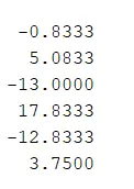
%right sided
n =

    1.0000    1.0000    1.0000    1.0000    1.0000    1.0000
   -5.0000   -4.0000   -3.0000   -2.0000   -1.0000         0
   12.5000    8.0000    4.5000    2.0000    0.5000         0
  -20.8333  -10.6667   -4.5000   -1.3333   -0.1667         0
   26.0417   10.6667    3.3750    0.6667    0.0417         0
  -26.0417   -8.5333   -2.0250   -0.2667   -0.0083         0

>> c=[0;0;1;0;0;0]

c =

     0
     0
     1
     0
     0
     0

>> e=inv(n)*c

e =

   -0.8333
    5.0833
  -13.0000
   17.8333
  -12.8333
    3.7500

>> f=[1,1,1,1,1,1;0,1,2,3,4,5;0,1/2,4/2,9/2,16/2,25/2;0,1/6,8/6,27/6,64/6,125/6;0,1/24,16/24,81/24,256/24,625/24;0,1/120,32/120,243/120,1024/120,3125/120]
%left sided
f =

    1.0000    1.0000    1.0000    1.0000    1.0000    1.0000
         0    1.0000    2.0000    3.0000    4.0000    5.0000
         0    0.5000    2.0000    4.5000    8.0000   12.5000
         0    0.1667    1.3333    4.5000   10.6667   20.8333
         0    0.0417    0.6667    3.3750   10.6667   26.0417
         0    0.0083    0.2667    2.0250    8.5333   26.0417

>> g=[0;0;1;0;0;0]

g =

     0
     0
     1
     0
     0
     0

>> d=inv(f)*g

d = 3.7500
  -12.8333
   17.8333
  -13.0000
    5.0833
%central difference
h =

    1.0000    1.0000    1.0000    1.0000    1.0000
   -2.0000   -1.0000         0    1.0000    2.0000
    2.0000    0.5000         0    0.5000    2.0000
   -1.3333   -0.1667         0    0.1667    1.3333
    0.6667    0.0417         0    0.0417    0.6667

>> o=[0;0;1;0;0]

o =

     0
     0
     1
     0
     0

>> p=inv(h)*o

p =

   -0.0833
    1.3333
   -2.5000
    1.3333
   -0.0833


    3.7500
  -12.8333
   17.8333
  -13.0000
    5.0833
   -0.8333

MAIN CODE

clear all
close all
clc
x=pi/3;
%range of dx
dx=linspace(pi/30,pi/300,20);
for i=1:length(dx)
    central_differ(i)=forth_order_central_diff(x,dx(i));
    right(i)=forth_order_right_diff(x,dx(i));
    left(i)=forth_order_left_diff(x,dx(i));
end
figure(1)
loglog(dx,central_differ,'r')
hold on
loglog(dx,right,'y')
hold on
loglog(dx,left,'g')
xlabel('dx')
ylabel('trucating error')
title('dx vs error')
legend('central','right sided','left sided','location','north')

CENTRAL DIFFERENCE

function error_central_diff=forth_order_central_diff(x,dx)
%analytical derivative = exp(x)*cos(x)
%f''(x)=-2*exp(x)*sin(x)
analytical=-2*(exp(x))*(sin(x));
%numerical derivative
a1=(0.0833333333333333333*(exp(x-(2*dx)))*cos(x-(2*dx)));
a2=(1.33333333333333333*(exp(x-dx))*cos(x-dx));
a3=(2.5000*(exp(x))*cos(x));
a4=(1.33333333333333333*(exp(x+dx))*cos(x+dx));
a5=(0.08333333333333333333*(exp(x+(2*dx)))*cos(x+(2*dx)));
central_diff=(-a1+a2-a3+a4-a5)/((dx)^2);
%error
error_central_diff=abs(analytical-central_diff);
end

LEFT DIFFERENCE

function error_left_diff=forth_order_left_diff(x,dx)
%analytical derivative = exp(x)*cos(x)
%f''(x)=-2*exp(x)*sin(x)
analytical=-2*(exp(x))*(sin(x));
%numerical derivative
a6=(0.833333333333333333*(exp(x-(5*dx)))*cos(x-(5*dx)));
a5=(5.0833333333333333333*(exp(x-(4*dx)))*cos(x-(4*dx)));
a4=(13.0000*(exp(x-(3*dx)))*cos(x-(3*dx)));
a3=(17.833333333333333333*(exp(x-(2*dx)))*cos(x-(2*dx)));
a2=(12.833333333333333333*(exp(x-dx))*cos(x-dx));
a1=(3.7500*(exp(x))*cos(x));
left_diff=(a1-a2+a3-a4+a5-a6)/((dx)^2);
%error
error_left_diff=abs(analytical-left_diff);
end

RIGHT DIFFERENCE

function error_right_diff=forth_order_right_diff(x,dx)
%analytical derivative = exp(x)*cos(x)
%f''(x)=-2*exp(x)*sin(x)
analytical=-2*(exp(x))*(sin(x));
%numerical derivative
c6=(0.833333333333333333*(exp(x+(5*dx)))*cos(x+(5*dx)));
c5=(5.0833333333333333333*(exp(x+(4*dx)))*cos(x+(4*dx)));
c4=(13.0000*(exp(x+(3*dx)))*cos(x+(3*dx)));
c3=(17.833333333333333333*(exp(x+(2*dx)))*cos(x+(2*dx)));
c2=(12.833333333333333333*(exp(x+dx))*cos(x+dx));
c1=(3.7500*(exp(x))*cos(x));
right_diff=(c1-c2+c3-c4+c5-c6)/((dx)^2);
%error
error_right_diff=abs(analytical-right_diff)
end

PLOT

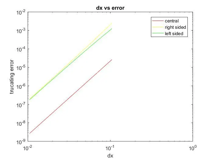
As we can see the error in the central scheme is less than the error in the skewed scheme. At the start of the curve right and left errors of left and right are similar. As dx increases error in the right-skewed scheme increases more than the left-skewed scheme.

We cant use central schemes when we have information that lies on either of the single sides. In that case, the skewed schemes are applicable. (For eg Boundary Conditions are one-sided).(although they are less accurate)

The dx must be kept small for greater accuracy.