Simulation of a 1D Super-sonic nozzle flow simulation using Macormack Method
Aim: to simulate the isentropic flow through a quasi 1D subsonic-supersonic nozzle numerically for both the conservation and non-conservation forms of the governing equations and solve them using MacCormack's technique in MATLAB.
Problem Description: The inlet of the nozzle is connected with the reservoir. The cross-sectional area of the reservoir is large tending towards infinity. As the area is large therefore Velocity is tending towards 0. The flow is locally subsonic in the converging section of the nozzle, sonic at the nozzle throat, and expands isentropically to the supersonic speed at the nozzle exit.
In this project, non-dimensional governing equations for the quasi-1D Converging-Diverging Nozzle in the conservative non-conservative form are discretized and solved with MacCormack's method.
The following results are obtained and compared for both forms:
1) Non-Dimensional mass flow rate across the nozzle for different time steps.
2) Transient variation of flow variables at the nozzle throat location.
3) Steady-State flow field across the nozzle.
4) Comparison of Steady-State mass flow rate along the nozzle x-direction for Conservative and Non-Conservative form.
5) Comparison of Steady-State flow variables at the throat location between Conservative, Non-Conservative form and analytical results.
6) Grid sensitivity flow.
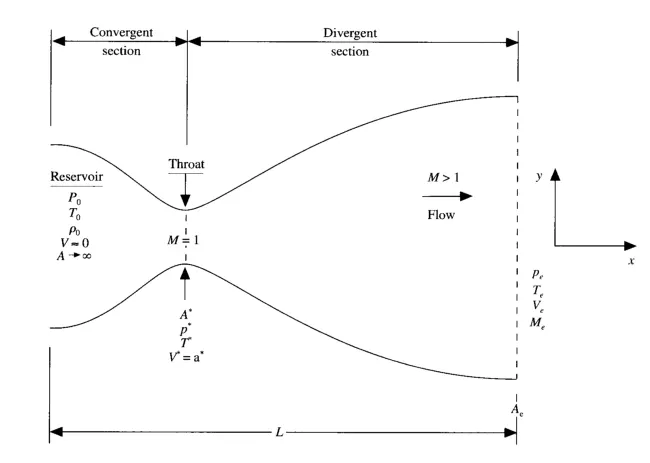
Non-Dimensional and Non-Conservative form of governing equation
Continuity Equation
`(partialrho')/(partialt') = (- rho'.(partialV')/(partialx'))-(rho'.V.'(partiallnA')/(partialx'))-(V'.(partialrho')/(partialx'))`
Momentum Equation
`(partialV')/(partialt') = (- V'.(partialV')/(partialx'))-1/gamma.((partialT')/(partialx'))+((T')/(rho').(partialrho')/(partialx'))`
Energy Equation
`(partialT')/(partialt') = - V'.(partialT')/(partialx')-(gamma-1).T'.((partialV')/(partialx')+V'.(partiallnA')/(partialx'))`
Non-Dimensional Conservative form of governing equation
Continuity Equation
`(del(rho'A'))/(delt') + (del(rho'A'V'))/(delx') = 0`
Momentum Equation
`(del(rho'A'V'))/(delt') + (del[rho'A'(V')^2 +(1/gamma)P'A'])/(delx') = (1/gamma)P'((delA')/(delx'))`
Energy Equation
`(del[rho'((e')/(gamma-1) + (gamma/2)(V')^2)A'])/(delt') + (del[rho'((e')/(gamma-1) + (gamma/2)(V')^2)V'A' + P'A'V'])/(delx') = 0`
where `gamma=1.4`.
MACCORMACK'S TECHNIQUE
Maccormacks technique is a variant of the Lax-Wendroff approach but it is simpler in its application. MacCormack's method is also an explicit finite-difference technique that is second-order-accurate in both space and time.
MacCormack's Method consists of two-step, First the Predictor step & then the Corrector step.
Let us consider a variable `f(x)` which can be any flow variable such as velocity, pressure, density, temperature, etc.
1. To start with MacCormack Method, First, we need the initial profile of the flow variables.
2. Predictor Step - Here we will calculate the time derivative using the initial profile of variables & the forward difference scheme.`((delf)/(dt))_p = (f(i+1)_("Initial") - f(i)_("Initial"))/(Deltax)`
3. Solution update for the predictor step
`f_p = f_(Initial) + ((delf)/(delt))_p * Deltat`.
`f_p` = value of flow variable at the predicted step.
`f_("Initial")`= Intial value of the flow variable.
`delt` = Time Step size.
4. Corrector Step - Here we will calculate the time derivative using the predicted profile of variables & the backward difference scheme.
`((delf)/(dt))_c = (f(i)_p - f(i-1)_p)/(Deltax)`
5. Average time derivative calculation.
`((delf)/(dt))_(avg) = 0.5(((delf)/(dt))_p +((delf)/(dt))_c )`
6. Final Solution update for the next time step.
`(f_i)^(n+1) = (f_(Initial))^n + ((delf)/(delt))_(avg) * Deltat`
`(f_i)^(n+1)` = value of solution variable at the next time step
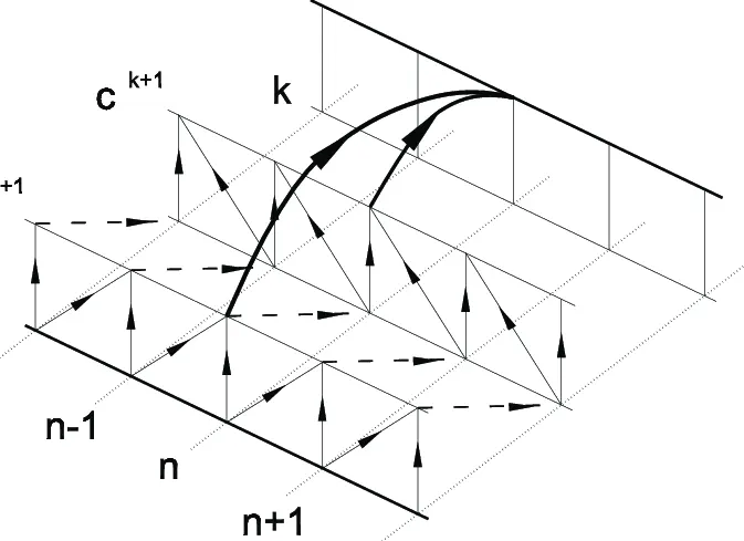
Stencil for the MacCormack method: n is the index for space, k for time; p is the predictor step, c is the corrector step.
Time Step Size Calculation
`delt = CFL((delx)/(a + v))`
`delt =` time step size
`delx`= minimum mesh size
a = local speed of sound inside the nozzle
v = local flow speed inside the nozzle.
`a = sqrt(T')`
`T'`= Local flow temperature inside the nozzle`delt` will be calculated for each and every grid point, from i = 1 to i = N based on the local flow and sound speed and minimum value of time step size will be chosen for the next time marching step.
`delt = "minimum"(delt_1,delt_2,delt_3,delt_4....... delt_n)`
Nozzle Shape and Initial conditions
The nozzle shape A=A(x), is specified and held fixed independent of time. For the case, we choose the parabolic area distribution given by `A=1+2.2(x-1.5)^2 0<=x<=3`
To start with the time marching calculations we must stipulate initial conditions for `rho`, T, and `V` as a function of x at time t=0.In theory, these initial conditions may be purely arbitrary but in practice, there are two reasons to choose an initial condition intelligently:
1)The closer the initial condition is to the final steady-state answer, the faster the time marching procedure will converge, and hence shorter will be the computer execution time.
2) If the initial conditions are too far away from reality, the initial timewise gradients at early time steps can become very large.
Therefore we know that `rho` and `T` decrease and `V` increases as the flow expands in the nozzle. Hence we choose initial conditions that qualitatively behave in the same fashion.
`rho=1-0.3146x`
`T=1-0.2314x`
`V=(0.1+1.09x)T^(1/2)` at t=0
Boundary Condition
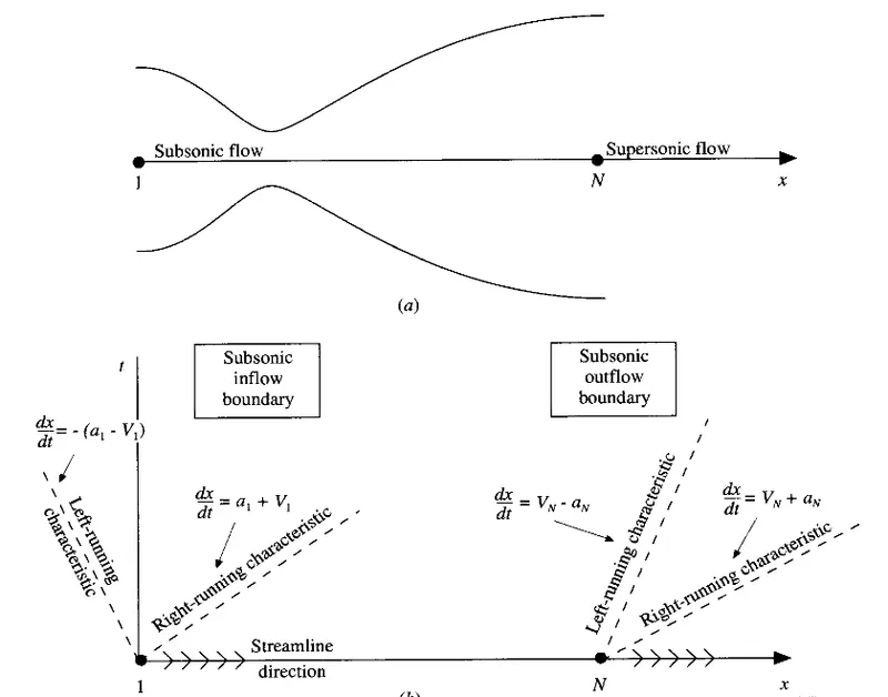
Unsteady, Inviscid flow is governed by hyperbolic equations, and therefore for 1D unsteady flow there exist two real characteristic lines through any point in xt plane. Physically these two characteristics represent infinitely weak Mach waves that are propagating upstream and downstream. Both Mach waves are traveling at the speed of sound 'a'. Let's have a look at the image below where we have a converging-diverging nozzle with xt plane drawn below it. This image will help us to define inlet and outlet boundary conditions.
The method of characteristics tells us that at a boundary where one characteristic propagates into the domain, then the value of one variable must be specified at that boundary and if one characteristics line propagates out of the domain, then the value of another flow variable must be extrapolated from the inside domain during the time marching solution.
Inlet Boundary Condition:
We can see that the local flow velocity at the inlet (point 1) is less than sound i.e subsonic(a<1). The match wave traveling towards left relative to fluid at the speed of sound easily works its way upstream against low subsonic flow, which moves from left to right. Hence left running characteristics are shown as `a_1-v_1`(relative to the fixed nozzle).
Since the calculated domain is contained between left and right grid points 1 to N then at point 1 we see the left running characteristic is running out of the domain.
As the fluid and mach wave, both are running towards the right therefore the right running characteristic is described by the combined velocity of `V_1+a_1`.
At inlet 1 we must specify the value of two dependent flow variables as one characteristic line and streamline entering into the domain and one flow variable must be extrapolated from the inside domain as one characteristic line going out from the inlet.
`rho_1' = 1` [Fixed value at the inlet]
`T_1' = 1` [Fixed value at the inlet]
`v_1=2*v_2 - v_3` [Extrapolated from the inside domain]
velocity is chosen to be float at the inlet because on a physical basis we know the mass flow through the nozzle must be allowed to adjust to the proper steady-state and allowing `V_1'` to adjust based on the flow field growth in time is most sensible. Since point 1 is viewed as the reservoir, we stipulate density and temperature value at point 1 to be their respective stagnation value `rho_o` & `T_o`respectively.
Outlet Boundary condition:
Supersonic outflow point(N). At N left running characteristics propagate left at the speed of sound 'a'. However the flow at the outlet is supersonic (v > a), the left running characteristics is carried downstream by the flow at a speed `v_n -a_n`, the right running characteristics propagates right at the speed of sound 'a' hence it is swept at a speed of `v_n + a_n`. So at the outlet both left and right running characteristics propagate out of the domain, so does the streamline at point N.
Hence at the outlet(point N), We must extrapolate all flow variables from the inside domain as both characteristic lines & streamline are going out from the outlet.
`v_n = 2v_(n-1) - v_(n-2)` [Floating]
`rho_n = 2rho_(n-1) - rho_(n-2)` [Floating]
`T_n = 2T_(n-1) -T_(n-2)` [Floating]
FUNCTION CODE FOR NON-CONSERVATION FORM
function [v,p,T,mach,mass_flo,rho,rho_throat,p_throat,v_throat,T_throat,mach_throat,mass_flo_throat]=non_conservative_form(n,x,dx,gma,CFL,nt)

% initial profile
%all flow variables in non-dimensional form
rho=1-0.3146*x;           %density
T=1-0.2314*x;             %temperature
v=(0.1+1.09*x).*T.^0.5;   %velocity
A=1+2.2*(x-1.5).^2;       %converging-diverging area

mass_flo_initial=rho.*A.*v; %mass flow rate
throat=find(A==1);        %find throat location
total_sim_time=0;         %initial flow time

%Solving descritized equations non-conservation form

%Macormack method
for k=1:nt %time marching

    % Storing initial data
    T_old=T;
    v_old=v;
    rho_old=rho;

    % calculating time step
    dt=min((CFL.*dx)./(sqrt(T)+v));

    % Predictor method
    for j=2:n-1

        dvdx=(v(j+1)-v(j))/(dx);

        drhodx=(rho(j+1)-rho(j))/(dx);

        dTdx=(T(j+1)-T(j))/(dx);

        dlnAdx=(log(A(j+1))-log(A(j)))/dx;

        %continuity equation
        drhodt_p(j)=-rho(j)*dvdx-rho(j)*v(j)*dlnAdx-v(j)*drhodx;

        %momentum equation
        dvdt_p(j)=-v(j)*dvdx-(1/gma)*(dTdx+(T(j)/rho(j))*drhodx);

        %energy equation
        dTdt_p(j)=-v(j)*dTdx-(gma-1)*T(j)*(dvdx+v(j)*dlnAdx);

    end
    for j=2:n-1
            %solution update
        v(j)=v(j)+dvdt_p(j)*dt;
        rho(j)=rho(j)+drhodt_p(j)*dt;
        T(j)=T(j)+dTdt_p(j)*dt;
    end
    %corrector method
    for j=2:n-1

        dvdx=(v(j)-v(j-1))/(dx);

        drhodx=(rho(j)-rho(j-1))/(dx);

        dTdx=(T(j)-T(j-1))/(dx);

        dlnAdx=(log(A(j))-log(A(j-1)))/dx;

        %continuity equation
        drhodt_c(j)=-rho(j)*dvdx-rho(j)*v(j)*dlnAdx-v(j)*drhodx;

        %momentum equation
        dvdt_c(j)=-v(j)*dvdx-(1/gma)*(dTdx+(T(j)/rho(j))*drhodx);

        %energy equation
        dTdt_c(j)=-v(j)*dTdx-(gma-1)*T(j)*(dvdx+v(j)*dlnAdx);
    end

    %average derivative
    dvdt=0.5*(dvdt_c+dvdt_p);
    drhodt=0.5*(drhodt_c+drhodt_p);
    dTdt=0.5*(dTdt_c+dTdt_p);

    %Solution Update
    for i=2:n-1
        v(i)=v_old(i)+dvdt(i)*dt;
        rho(i)=rho_old(i)+drhodt(i)*dt;
        T(i)=T_old(i)+dTdt(i)*dt;
    end
    %Boundary Condition
    %inlet
    rho(1)=1;         %fixed
    T(1)=1;           %fixed
    v(1)=2*v(2)-v(3); %extrapolated
    % outlet
    %extrapolated from inside
    v(n)=2*v(n-1)-v(n-2);
    rho(n)=2*rho(n-1)-rho(n-2);
    T(n)=2*T(n-1)-T(n-2);

        %Calculating the non-dimensional mass flow rate, Pressure, Mach_no
        mass_flo=rho.*A.*v;
        p=rho.*T;
        mach=v./sqrt(T);

        %calculating the non-dimensional variables at nozzle throat
        rho_throat(k)=rho(throat);
        v_throat(k)=v(throat);
        T_throat(k)=T(throat);
        p_throat(k)=p(throat);
        mass_flo_throat(k)=mass_flo(throat);
        mach_throat(k)=mach(throat);

        %updating total flow time
        total_sim_time=total_sim_time+dt;
        dvdt_throat(k)=dvdt(throat);
        drhodt_throat(k)=drhodt(throat);

        figure(1)
        if k==1
            plot(x,mass_flo_initial,'color','K','LineWidth',1.3,'LineStyle','--')
            hold on
            elseif k==50
            plot(x,mass_flo,'color','m','LineWidth',1.3)
            hold on
            elseif k==100
            plot(x,mass_flo,'color','r','LineWidth',1.3)
            hold on
            elseif k==150
            plot(x,mass_flo,'color','g','LineWidth',1.3)
            hold on
        elseif k==200
            plot(x,mass_flo,'color','b','LineWidth',1.3)
            hold on
        elseif k==700
            plot(x,mass_flo,'color','y','LineWidth',1.3)
            hold on
        end


end

        title('Mass flow rate distribution across the nozzle[Non-Conservation form]')
        xlabel('Nozzle x-distance')
        ylabel('Non Dimensional mass flow rate')
        legend('1^s^t timestep','50^t^h timestep','100^t^h timestep','150^t^h timestep','200^t^h timestep','700^t^h timestep')
        axis([0 3 0.1 2])
        grid minor;
% plotting the density, velocity time derivative variation with time at the
% nozzle throat
figure(2)
plot(linspace(1,nt,nt),dvdt_throat,'k','linewidth',1.3);
hold on
plot(linspace(1,nt,nt),drhodt_throat,'g','linewidth',1.3);
title('time derivative of velocity and density[non conservative form]')
xlabel('no of steps')
ylabel('residuals')
legend('$dv/dt$','$drho/dt$');
grid minor;

%plotting mach number and density with nozzle length
figure(3)
plot(x,rho,'k','Linewidth',1.3);
xlabel('Nozzle X-direction')
ylabel('non-dimensional density')
yyaxis right
plot(x,mach,'r','Linewidth',1.3);
ylabel('Non-Dimensional mach')
grid minor;
title('Steady State Density & Mach No. across Nozzle[non conservative form]')
legend('Density','Mach Number');
%Printing total flow time
sprintf('total flow time for non conservative form=%.2f seconds',total_sim_time)
grid minor
end
The use of Governing Equations in conservation form:
Theoretically, either form of the governing flow equations is a suitable representation of the fundamental physical principles of mass conservation, Newton's third law, and energy conservation. However, in CFD, there are some good numerical reasons to use one form over the other for the solution of certain flow problems.
An important note is conservation form is more suitable in shock capturing than non-conservation.
The governing equations for quasi one-dimensional flow can be expressed in a more generic form by defining the elements as the solution vector U the flux vector F and the source term J as follows.
`U1=rho'A'`
`U2=rho'A'V'`
`U3=rho'[(e')/(gamma-1)+(gamma)/(2(V')^2]A'`
`F1=rho'A'V'`
`F2=rho'A'(V')^2+1/gamma*rho'A'`
`F3=rho'((e')/(gamma-1)+(gamma)/(2)(V')^2))A'V'+P'A'V'`
J2=`1/gammaP'(deltaA')/(deltax')`with these elements governing equations can be written as;
Continuity:`(deltaU1)/(deltat')=-(deltaF1)/(deltax')`
Momentum:`(deltaU2)/(deltat')=-(deltaF2)/(deltax')+J_2`
Energy:`(deltaU3)/(deltat')=-(deltaF3)/(deltax')`
In the conservative form of governing equations the dependent variables to obtain the primitive variables(rho,V,P,T etc...) we must decode the elements U1,U2,U3 as follows.
`rho'=U1/A'`
`V'=U2/U1`
`T'=`e'-(gamma-1)(U3)/(U2)-(gamma)/(2)(V')^2`
P'=rho'T'
Therefore after we obtain U1,U2 and U3 at each time step from the numerical solution of equations we can immediately calculate the corresponding primitive variables at each time step rho',V',T' and P' from equations.
Pure form of flux vector is given by:
F1=U2
F2=`(U2^2)/(U1)+(gamma-1)/(gamma)[U3-(gamma)/(2)(U2^2)/(U1^2)]`
F3=`gamma(U2U3)/(U1)-gamma(y-1)/(2)(U2^2)/(U1^2)`
J2=`(gamma-1)/(gamma)(U3-(gamma)/2(U2^2)/(U1))(delta(lnA')/(deltax'))`
This is the pure form of governing equation in conservative form.
Initial conditions:
for `0<x'0.5: rho'=1.0 and T' =1.0`
for `0.5<1.5: rho'=1.0-0.366(x'-0.5)` and `T'=1.0-0.167(x'-0.5)`
for `1.5<x'<3.0: rho'=0.634-0.3879(x'-1.5)` and `T'=0.833-0.3507(x'-1.5)` .
for the initial condition only,lets assume a constant mass flow through the nozzle and calculate V as,
`V'=(U2)/(rho'A')=(0.59)/(rho'A')`
The value of 0.59 is chosen for U2 because it is the closest to the exact analytical value of the steady state mass flow (i.e)=0.579.
Boundary conditions:
Subsonic inlet boundary (at node 1)
Two properties are held fixed and one is allowed to float rho and T are fixed at inflow boundary both equal to 1 and allowing V to float.`(U1_1)_(i=1)=rho'A'_(i=1)``(U2)_(i=2)=2(U2)_(i=2)-(U2)_(i=3)``(U3)_(i=1)=rho'[(e')/(gamma-1)+gamma/2V'^2]A'`
Supersonic outflow boundary(at node N)
All properties are allowed to float:
`(U1)_n=2(U1)_(n-1)-(U1)_(n-1_`
`(U2)_n=2(U2)_(n-1)-(U2)_(n-1_`
`(U3)_n=2(U3)_(n-1)-(U3)_(n-1_`
FUNCTION CODE FOR CONSERVATION FORM
function [v,p,T,mach,mass_flo,rho,rho_throat,p_throat,v_throat,T_throat,mach_throat,mass_flo_throat]=conservative_form(n,x,dx,gma,CFL,nt)

% initial profile
%all flow variables in non-dimensional form
for i=1:n
    if x(i)<=0.5
rho(i)=1;           %density
T(i)=1;             %temperature
    elseif (x(i)>0.5 && x(i)<=1.5)
        rho(i)=1-0.366*(x(i)-0.5);
        T(i)=1-0.167*(x(i)-0.5);
    elseif (x(i)>1.5&&x(i)<=3.5)
        rho(i)=0.634-0.3879*(x(i)-1.5);
        T(i)=0.833-0.3507*(x(i)-1.5);
    end

end

A=1+2.2*(x-1.5).^2;        %converging diverging area
v=0.59./(rho.*A);         %velocity

%mass_flo_initial=rho.*A.*v; %mass flow rate % In conservation form flow rate = U2
throat=find(A==1);        %find throat location
total_sim_time=0;         %initial flow time

U1=rho.*A;
U2=rho.*A.*v;
U3=rho.*A.*(T/(gma-1)+(0.5*gma.*v.^2));

%Solving descritized equations conservation form

%Macormack method
for z=1:nt %time marching

    % Storing initial data
    U1_old=U1;
    U2_old=U2;
    U3_old=U3;

    % calculating time step
    dt=min((CFL.*dx)./(sqrt(T)+v));
    %calculating initial flux vector

    F1=U2;
    F2=((U2.^2)./U1)+((gma-1)/gma)*(U3-(gma/2)*(U2.^2)./U1);
    F3=((gma.*U2.*U3)./U1)-(gma*(gma-1)/2)*((U2.^3)./(U1.^2));

    % Predictor method
    for j=2:n-1
        %Source term
        J=(1/gma)*rho(j)*T(j)*((A(j+1)-A(j))/dx);

        %continuity equation
        dU1_dt_p(j)=-((F1(j+1)-F1(j))/dx);

        %momentum equation
        dU2_dt_p(j)=-((F2(j+1)-F2(j))/dx)+J;

        %energy equation
        dU3_dt_p(j)=-((F3(j+1)-F3(j))/dx);

        %updating the solution vector
        U1(j)=U1(j)+dU1_dt_p(j)*dt;
        U2(j)=U2(j)+dU2_dt_p(j)*dt;
        U3(j)=U3(j)+dU3_dt_p(j)*dt;
    end

    %correcting flux vector
    F1=U2;
    F2=((U2.^2)./U1)+((gma-1)/gma)*(U3-(gma/2)*(U2.^2)./U1);
    F3=((gma.*U2.*U3)./U1)-(gma*(gma-1)/2)*((U2.^3)./(U1.^2));
    %calculating premitive variables
        rho=U1./A;
        v=U2./U1;
        T=(gma-1)*((U3./U1)-((gma/2)*(v.^2)));
        p=rho.*T;

        %corrector step
        for k=2:n-1
        %Source term
        J=(1/gma)*rho(k)*T(k)*((A(k)-A(k-1))/dx);

        %continuity equation
        dU1_dt_c(k)=-((F1(k)-F1(k-1))/dx);

        %momentum equation
        dU2_dt_c(k)=-((F2(k)-F2(k-1))/dx)+J;

        %energy equation
        dU3_dt_c(k)=-((F3(k)-F3(k-1))/dx);
        end

    %average derivative
    dU1_dt=0.5*(dU1_dt_c+dU1_dt_p);
    dU2_dt=0.5*(dU2_dt_c+dU2_dt_p);
    dU3_dt=0.5*(dU3_dt_c+dU3_dt_p);

    %calculating corrected solution vector
    for m=2:n-1
        U1(m)=U1_old(m)+dU1_dt(m)*dt;
        U2(m)=U2_old(m)+dU2_dt(m)*dt;
        U3(m)=U3_old(m)+dU3_dt(m)*dt;
    end

        %calculating corrected primitive non-dimensional variable for next
        %time step
        rho=U1./A;
        %v=U1./U2; % v = U2/U1
        v=U2./U1;
        T=(gma-1)*((U3./U1)-((gma/2)*(v.^2)));
        p=rho.*T;
        mass_flo=U2;
        mach=(v./sqrt(T));

    %Boundary Condition
    %inlet
    U1(1)=rho(1)*A(1);              %fixed value
    U2(1)=2*U2(2)-U2(3);            %extrapolated
    U3(1)=U1(1)*((T(1)/(gma-1))+((gma/2)*(v(1)^2)));

    % outlet
    %extrapolated from the inside domain
    U1(n)=2*U1(n-1)-U1(n-2);
    U2(n)=2*U2(n-1)-U2(n-2);
    U3(n)=2*U3(n-1)-U3(n-2);

        %calculating the non-dimensional variables at nozzle throat
        rho_throat(z)=rho(throat);
        v_throat(z)=v(throat);
        T_throat(z)=T(throat);
        p_throat(z)=p(throat);
        mass_flo_throat(z)=mass_flo(throat);
        mach_throat(z)=mach(throat);

                %updating total flow time
        total_sim_time=total_sim_time+dt;
          %plotting the numerical results
          %non dimensional mass flow rate at the different time steps
        figure(6)
        if z==1
            plot(x,mass_flo,'color','K','LineWidth',1.3,'LineStyle','--')
            hold on
            elseif z==50
            plot(x,mass_flo,'color','m','LineWidth',1.3)
            hold on
            elseif z==100
            plot(x,mass_flo,'color','r','LineWidth',1.3)
            hold on
            elseif z==200
            plot(x,mass_flo,'color','g','LineWidth',1.3)
            hold on
        elseif z==400
            plot(x,mass_flo,'color','b','LineWidth',1.3)
            hold on
        elseif z==700
            plot(x,mass_flo,'color','y','LineWidth',1.3)
            hold on
        end


end

        title('Mass flow rate distribution across the nozzle[Conservation form]')
        xlabel('Nozzle x-distance')
        ylabel('Non Dimensional mass flow rate')
        legend('1^s^t timestep','50^t^h timestep','100^t^h timestep','200^t^h timestep','400^t^h timestep','700^t^h timestep')
        axis([0 3 0.1 2])
        grid minor
%Printing total flow time
sprintf('total flow time for non conservative form=%.2f seconds',total_sim_time)
end
.......................................................................MAIN CODE..............................................................................
clear all
close all
clc
%inputs
n=31;              %mesh points
x=linspace(0,3,n); %1-D mesh
dx=x(2)-x(1);      %grid spacing
gma=1.4;           %gas constant
nt=1400;            %no of time step
CFL=0.5;           %CFL number
%Non Conservative form
[v,p,T,mach,mass_flo,rho,rho_throat,p_throat,v_throat,T_throat,mach_throat,mass_flo_throat]=non_conservative_form(n,x,dx,gma,CFL,nt);

%plotting mach number and density with nozzle length
figure(3)
plot(x,rho,'k','Linewidth',1.3);
xlabel('Nozzle X-direction')
ylabel('non-dimensional mach no.')

yyaxis right
plot(x,mach,'r','Linewidth',1.3);
ylabel('Non-Dimensional mach')
grid minor;

title('Steady State Density & Mach No. across Nozzle[non conservative form]')
legend('Density','Mach Number');

%Printing total flow time
% sprintf('total flow time for non conservative form=%.2f seconds',total_sim_time)

%plotting time wise variation of non-dimensional primitive variables at
% %nozzle throat
% hold on
figure(4)
%density
subplot(4,1,1)
plot(linspace(1,nt,nt),rho_throat,'color','r','linewidth',1.5)
ylabel('density')
axis([0 1000 0 1.4]);
grid minor;
title('Non dimensional flow variable variation with time at nozzles throat [Non conservative time]')
%temperature
subplot(4,1,2)
plot(linspace(1,nt,nt),T_throat,'color','g','linewidth',1.5)
ylabel('temperature')
axis([0 1000 0.5 1]);
grid minor;
%pressure
subplot(4,1,3)
plot(linspace(1,nt,nt),p_throat,'color','b','linewidth',1.5)
ylabel('pressure')
axis([0 1000 0.3 1.2]);
grid minor;
%Mach Number
subplot(4,1,4)
plot(linspace(1,nt,nt),mach_throat,'color','y','linewidth',1.5)
xlabel('time step')
ylabel('Mach Number')
axis([0 1000 0.5 1.5]);
grid minor;


%plotting steady state field of non-dimensional primitive variables across
%nozzle

% hold on
figure(5)
%density
subplot(4,1,1)
plot(x,rho,'color','m','linewidth',1.5)
ylabel('density')
axis([0 3 0 1]);
grid minor;
title('Steady-State flow field vs Nozzle x-direction [Non-conservative form]')
%Temperature
subplot(4,1,2)
plot(x,T,'color','c','linewidth',1.5)
ylabel('Temperature')
axis([0 3 0 1]);
grid minor;
%Pressure
subplot(4,1,3)
plot(x,p,'color','g','linewidth',1.5)
ylabel('Pressure')
axis([0 3 0 1]);
grid minor;
%Mach Number
subplot(4,1,4)
plot(x,mach,'color','y','linewidth',1.5)
ylabel('Mach no.')
axis([0 3 0 4]);
grid minor;

mass_flo_rate_NC=mass_flo;
rho_NC=rho_throat;
p_NC=p_throat;
T_NC=T_throat;
mach_NC=mach_throat;

%Conservative Form
[v,p,T,mach,mass_flo,rho,rho_throat,P_throat,v_throat,T_throat,mach_throat,mass_flo_throat]=conservative_form(n,x,dx,gma,CFL,nt);
%plotting time wise variation of non-dimensional primitive variables at
%nozzle throat
%hold on
figure(7)
%density
subplot(4,1,1)
plot(linspace(1,nt,nt),rho_throat,'color','b','linewidth',1.5)
ylabel('density')
axis([0 1000 0 1.4]);
grid minor;
title('Non dimensional flow variable variation with time at nozzles throat [conservative time]')
%temperature
subplot(4,1,2)
plot(linspace(1,nt,nt),T_throat,'color','m','linewidth',1.5)
ylabel('temperature')
axis([0 1000 0.5 1]);
grid minor;
%pressure
subplot(4,1,3)
plot(linspace(1,nt,nt),P_throat,'color','g','linewidth',1.5)
ylabel('pressure')
axis([0 1000 0.3 1.2]);
grid minor;
%Mach Number
subplot(4,1,4)
plot(linspace(1,nt,nt),mach_throat,'color','y','linewidth',1.5)
xlabel('time step')
ylabel('Mach Number')
axis([0 1000 0.5 1.5]);
grid minor;


%plotting steady state field of non-dimensional primitive variables across
%nozzle
%
% hold on
figure(8)

%density
subplot(4,1,1)
plot(x,rho,'color','m','linewidth',1.5)
ylabel('density')
axis([0 3 0 1]);
grid minor;
title('Steady-State flow field vs Nozzle x-direction [Conservative form]')
%Temperature
subplot(4,1,2)
plot(x,T,'color','c','linewidth',1.5)
ylabel('Temperature')
axis([0 3 0 1]);
grid minor;
%Pressure
subplot(4,1,3)
plot(x,p,'color','g','linewidth',1.5)
ylabel('Pressure')
axis([0 3 0 1]);
grid minor;
%Mach Number
subplot(4,1,4)
plot(x,mach,'color','y','linewidth',1.5)
ylabel('Mach.No')
axis([0 3 0 4]);
grid minor;

mass_flo_rate_C=mass_flo;
rho_C=rho_throat;
P_C=P_throat;
T_C=T_throat;
mach_C=mach_throat;

%Comparison of normalized steady-state mass-flow rate across the nozzle
%between conservative and non-conservative form

%analytical non dimensional mass flow ratethrough the nozzle =0.590
mass_flo_rate_analytical=0.59*ones(1,n);

figure(9)
% hold on
plot(x,mass_flo_rate_NC,'r','Linewidth',1.5);
hold on
plot(x,mass_flo_rate_C,'k','Linewidth',1.5);
hold on
plot(x,mass_flo_rate_analytical,'g','Linewidth',1.5,'Linestyle','--');
grid minor;
legend('Non-conservative form','Conservative form','analytical')
xlabel('Nozzle X-direction')
ylabel('Non dimensional mass flow rate')
title('Comparison of steady normalized mass flow rate of consevative and non-conservative form')
RESULTS
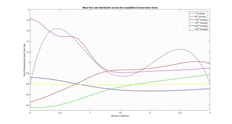
This graph shows the distribution of non-dimensional mass flow rate across the non-dimensional distance of the nozzle at different time steps across the nozzle. These are obtained by solving the non-conservative form of equations. There are 6 graphs at different time steps during the time marching solution. The dashed curve is mass distribution at 0th timestep i.e initial condition. The mass flow rate started to change from the 50th timestep and changes drastically at the 100th step due to the transient nature of the flow field variable across the nozzle. However, after 200 time-steps mass flow rate distribution begins to settle down and after 700 timesteps mass flow rate distribution across the nozzle becomes constant and converges.
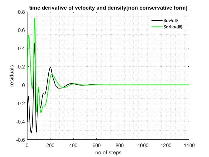
This graph shows the residuals with respect to the number of timesteps obtained by solving the non-conservation form of the equations. The time derivative of density and velocity are present LHS of continuity and momentum equation, As time progresses and as steady-state is approached, the RHS of continuity and momentum equation should approach 0. Velocity and density should not change with respect to time after steady-state. Since it is almost impossible to have right-hand-side(residuals) precisely 0 due to the numerical method.
At an early time derivatives of density and velocity is large, they oscillate in value. This oscillation is associated with the compression-expression waves propagating through the nozzle in the transient process.
After a time these derivatives settle down and approach a steady state. Although the absolute steady-state can't be reached with a finite amount of time.
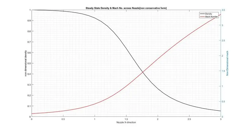
The above graph shows the non-dimensional Mach no. & non-dimensional Density variation across the non-dimensional distance of the nozzle obtained by solving the non-conservative form of equations. We can see the flow is subsonic in the nozzle converging section(x<1.6), the flow becomes sonic at the nozzle throat(x = 1.6), Flow goes supersonic in diverging section of the nozzle(x > 1.6). Density decreases as flow expand through the nozzle.
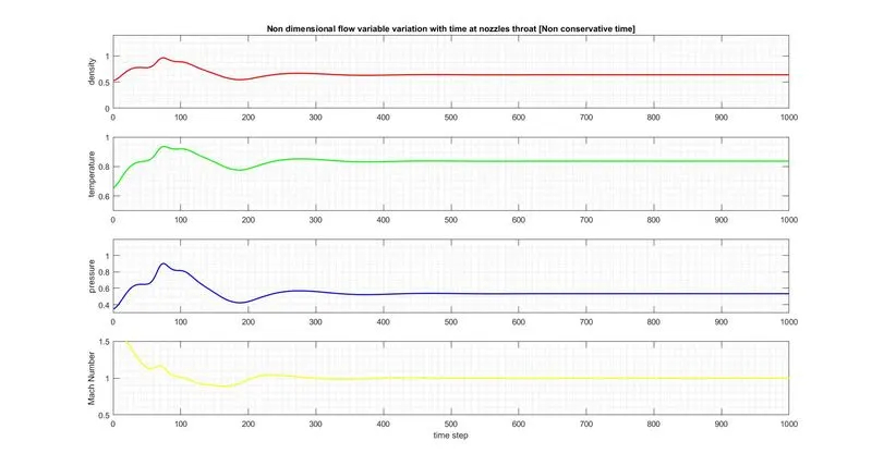
The above graph shows the non-dimensional Density, Temperature, Pressure & Mach No. transient variation at the nozzle's throat location obtained by solving the non-conservative form of equations. The largest change takes place at early times, the transient behavior can be seen. The magnitude of the initial change in variable depends on applied initial conditions. But after a long course of time, around ~ 400-time steps, change in the variable is getting relaxed, and a steady-state is achieved.
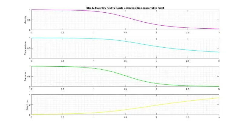
The above graph shows the steady-state field of non-dimensional Density, Temperature, Pressure & Mach No. across the direction of the nozzles obtained by solving the non-conservative form of equations. The results show good agreement with the analytical results qualitatively and quantitatively(analytical results are not shown in the graph but can be easily obtained). (Please refer to John D Anderson CFD book for the verification of results).
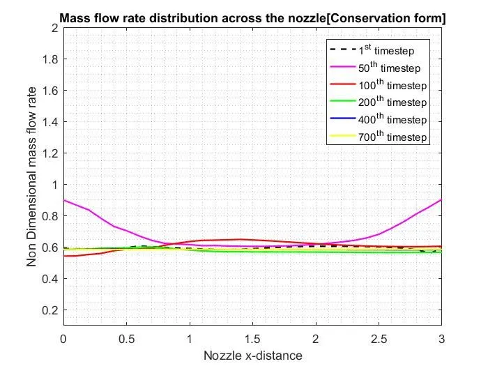
The above graph shows the instantaneous non-dimensional mass flow rate distribution across the non-dimensional distance of the nozzle at the different time steps obtained by solving the non0conservative form of equations. There are 6 curves, each at different times during the time marching solution. The dashed straight curve refers to the initial distribution(initial condition) of mass flow rate at time 0 second. The constant mass-flow rate = 0.59(close to analytical result) across the nozzle is assumed for the calculation of the non-conservative form of the equation. After the 700th time step, we can see the steady-state distribution of the mass-flow rate is achieved across the nozzle.
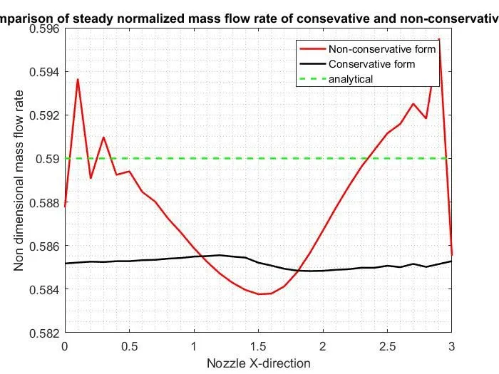
The above graph shows the steady-state mass flow rate profile(at a magnified scale) comparison between conservative and non-conservative forms numerical results after the 1400th time step when the convergence is achieved.
Although on large scales these variations are negligible but on a magnified scale we can see that the non-conservation form shows greater variation from analytical results than the conservation form. The conservation form performs better for stability and conserving the mass flow rate as in the conservation form of momentum equation, an emphasis is laid on mass flow rate in comparison to the non-conservation form.
| At nozzle throat (after 1400 timestep) | Density | Temperature | Pressure | Mach.No |
| non-conservative form(31 grid points) | 0.639 | 0.836 | 0.534 | 0.999 |
| non-conservative form(61 grid points) | 0.640 | 0.836 | 0.535 | 1.003 |
| conservative form(31 grid points) | 0.650 | 0.840 | 0.546 | 0.982 |
| non-conservative form(61 grid points) | 0.638 | 0.835 | 0.533 | 0.999 |
| analytical results | 0.634 | 0.838 | 0.528 | 1.000 |
Non-Conservative form numerical results are distinctly closer to the analytical results as compared with numerical results obtained from the conservative form of equations.
For the non-conservative form of numerical results, the mesh independence is achieved at 31 grid points itself which is not the case in numerical results obtained from the conservative form of equations.
After doubling the grid points numerical results obtained from the conservative form of equations are closer to the analytical results but still not as close as the non-conservative form of numerical results with half as many grid points.
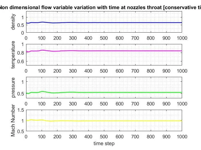
The above graph shows the non-dimensional Density, Temperature, Pressure & Mach No. transient variation at the nozzle's throat location obtained by solving the conservative form of equations. If we compare this with numerical results obtained from non-conservative form, Here we can notice initial gradients/changes are not that too high and the flow variable started converge after ~200 time steps whereas in the non-conservative form we can notice flow variable converges and reaches steady state solution at ~400 time steps. Here faster convergence can be seen because of using better initial conditions.
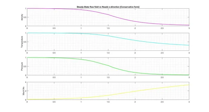
The results show good agreement with the analytical results qualitatively and quantitatively.
References:
Anderson, John D., Jr. Conputational Fluid Dynamics, The basics with applications, Chapter 7,Numerical Solutions of Quasi-One-Dimensional Nozzle Flows, page No:283-364.