FVM Literature Review

The transport equations governing fluid flow and heat transfer and the formal control volume can be solved numerically based on integration by Finite Volume Method.

The finite volume method (FVM) is a method for representing and evaluating partial differential equations in the form of algebraic equations. In the finite volume method, volume integrals in a partial differential equation that contain a divergence term are converted to surface integrals, using the divergence theorem. These terms are then evaluated as fluxes at the surfaces of each finite volume. Because the flux entering a given volume is identical to that leaving the adjacent volume, these methods are conservative. Another advantage of the finite volume method is that it is easily formulated to allow for unstructured meshes. The method is used in many computational fluid dynamics packages. "Finite volume" refers to the small volume surrounding each node point on a mesh.

Finite Volume Method vs Finite Difference Method

FDM is a differential scheme, that is an approximation of Taylor series expansion. We write the first order, second order differential in terms of the difference between two point values.

FVM is an integral scheme. Since we are integrating across the area, the chance of error is minimized.

FDM discretization is based upon the differential form of the PDE to be solved. FDM method stores the numerical solution on the nodes. FDM can only be applied to the Structured mesh.

FVM is based upon the integral form of the PDE to be solved. FVM method stores the numerical solution on the finite volume cell centroids. FVM can be applied to both Structured & Unstructured mesh.

The finite-volume method’s strength is that it only needs to do flux evaluation for the cell boundaries. This also holds for nonlinear problems, which makes it extra powerful for robust handling of (nonlinear) conservation laws appearing in transport problems.

Another advantage of the FVM method is that we don't need to care about the conservation of quantities as in FVM the conservation equations are already imbibed in the system while in FDM it is not the case.

If we take the example of the 1-D heat conduction equation

1-D linear heat conduction equation discretization

This is the general form of heat transport equation in the convective and diffusion form with variable `T`.

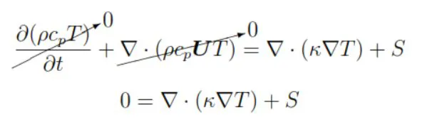
The convective term and time derivative terms are ignored.

so the equation becomes

for 1-D y,z terms are also ignored

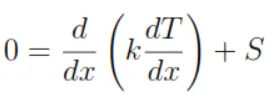
The above equation is 1D steady-state heat diffusion equation. This equation will be solved using the finite-volume method.

Finite Volume Method Discretization

Finite Volume Method requires integration and the application of boundary conditions. Rather than integrate the equation over the entire domain, the first stage in the finite volume method is to integrate the equation over a small piece of the domain. This piece is called a finite volume.

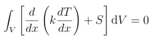
The integration of each term can be considered separately, as addition and integration are commutative operations.

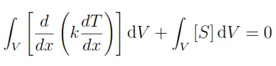
The second term in the above equation represents the heat source generated in the finite volume. Assume that the heat source is constant across the control volume, with a value of `¯S` (the volume average heat source). The second term in the finite volume integral can now be simplified.

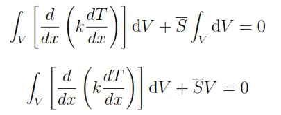
Note: Normally the source term present in our transport equation is linearized instead of considering the constant source term. The reason behind doing this to improve the stability of our numerical solution. By linearizing the source term, We can make the coefficient matrix diagonal dominance stronger. This helps in enhancing the convergence in CFD.

The first term in the above equation is the volume integral of the heat diffusion inside the control volume.

To evaluate this term, the divergence theorem is used.

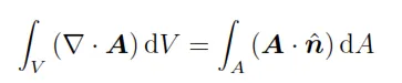
The divergence theorem states that the rate of accumulation of a vector field inside a control volume is equal to the flux of the vector field across the surfaces of the control volume.

The general form of divergence theorem applied over the vector field A is shown below.

In 1D, the divergence theorem can be written as:

Applying a 1D form of divergence theorem on our Heat equation will yield:

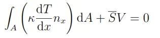
Physically, the above equation states that the flux of heat out of the cell by diffusion must balance the heat generated within the cell. The flow quantities (temperature, thermal conductivity, etc.) are constant on the cell face. Hence, the first integral can be simplified:

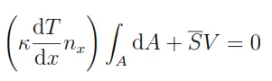
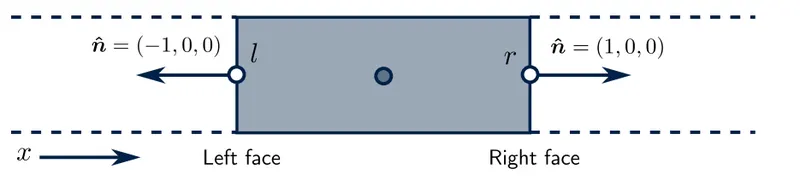
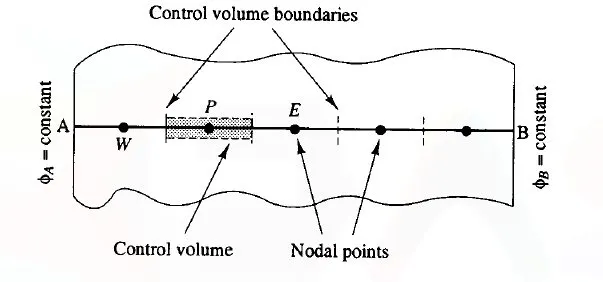
The figure shown above is our finite control volume with left face 'l' & right face 'r' & their unit normal vectors.Applying the integration limits from left to right face above equation can be written as:-

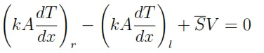
The above equation is the discretized form of the 1D heat-diffusion equation is valid for all cells in the mesh.

1D Convection Diffusion Heat Equation

Similarly, we can discretize the 1D convection-diffusion heat equation using the above method.

The above equation shows the integral form of the convection-diffusion heat equation & the below equation is the discretized form of it valid on cells in the mesh.

In the finite volume method, flow variables are calculated & stored at the cell centroid.

By looking at the Diffusion term of the above equation, we need the temperature gradient, conductivity on the cell left & right face & by looking at the Convection term of the above equation, We also need the value of velocity, temperature, thermal heat capacity & density on the cell left & right face.

Now to calculate these gradients & flow variables we need to use some type of interpolation from the neighboring cell centroid values. These schemes are known as interpolation schemes.

For the diffusion term, the Interpolation scheme used for the Diffusion term is the Central Difference scheme & for the convection term is the Linear Upwind scheme.

Flux Limiter

ϕf=ϕp+∇ϕp⋅r

ϕp - Value of flow variable on the cell centroid.

ϕf - Value of flow variable on the cell face.

∇ϕp- gradient of flow variable

r - Normal distance between cell face & cell centroid

Using the above expression, we can evaluate the flow variable on the cell faces.

If the gradient is too steep in a cell, then while doing a linear interpolation of the flow variables on the cell faces from the cell centroids, we might end up with an unphysical solution.

This is due to the fact that having steep gradients within the cell and doing linear interpolations we might end up having a cell face flow variable value greater than the flow variable value on the cell centroid. This is not physical and this leads to instability in the solution.

In order to prevent these instabilities, we will use Flux limiters.

ϕf=ϕp+γ⋅∇ϕp⋅r

0<γ<1

γ- flux limiter

Flux limiter ensures the value evaluated at the cell faces is bounded.

Gradient Scheme

We also need the gradient scheme in our CFD calculation. Gradient Scheme calculates the gradient of flow variable on the cell centroids. These gradients are required in the Linear Upwind Interpolation scheme, linearizing the source term & non-orthogonal corrector for diffusion term.