Week 7: Shock tube simulation project

Assignment name – Shock Tube simulation using Converge

Objective: -

• Setup a transient shock tube simulation
• Plot the pressure and temperature history in the entire domain - Explain the result
• Plot the cell count as a function of time - Explain the result

Introduction:

• The shock tube is an instrument used to replicate and direct blast waves at a sensor or a model in order to simulate actual explosions and their effects, usually on a smaller scale.
• A simple shock tube is a tube, rectangular or circular in cross-section, usually constructed of metal, in which a gas at low pressure and a gas at high pressure are separated using some form of diaphragm. See, for instance, texts by Soloukhin, Gaydon and Hurle, and Bradley.

Steps Required for this simulation

• Geometry
• Case setup
• Run the simulation in Cygwin
• Post process results in Para view

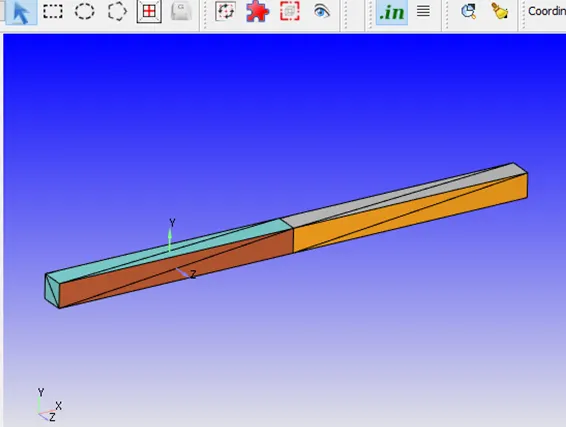
Geometry:

Import the STL file into the converge

Check the normal

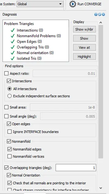
Check diagnosis if whether there is any fault in geometry and correct them

Diagnosis

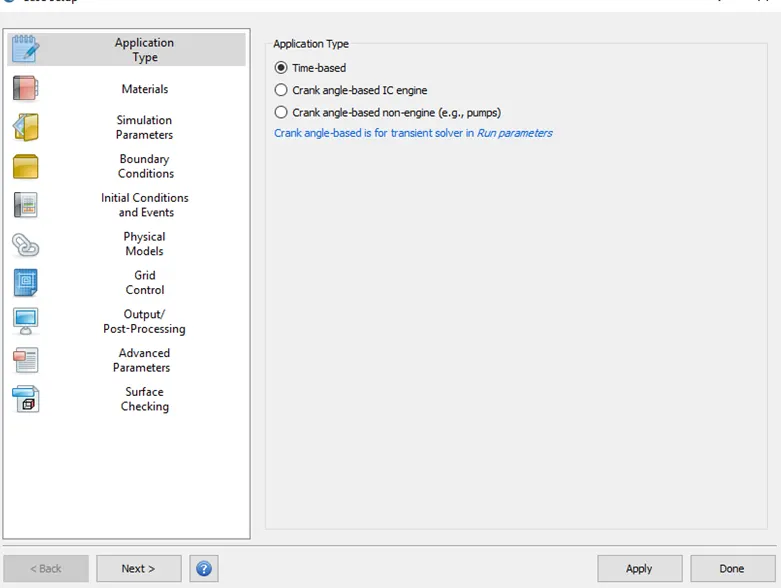
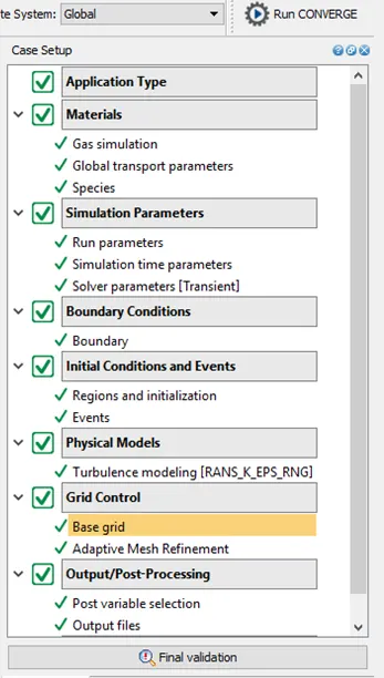
Case setup

Application Type

Application type: Time based- General flow

Materials : Air

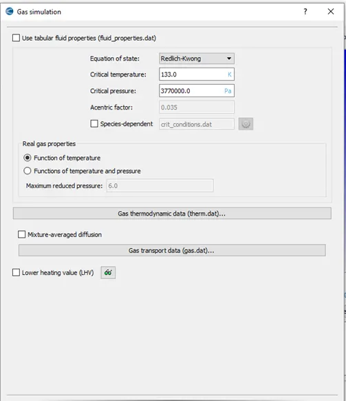
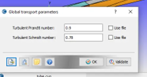
Global Transport parameters

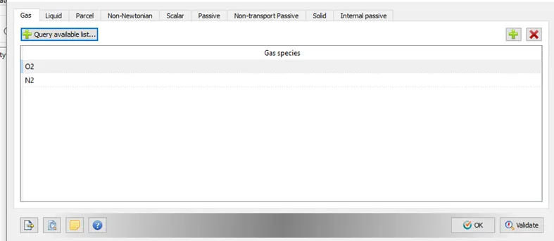
Species

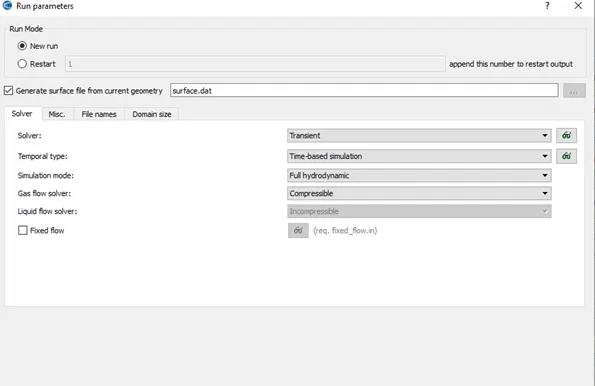
Run parameters

Slover: Transient

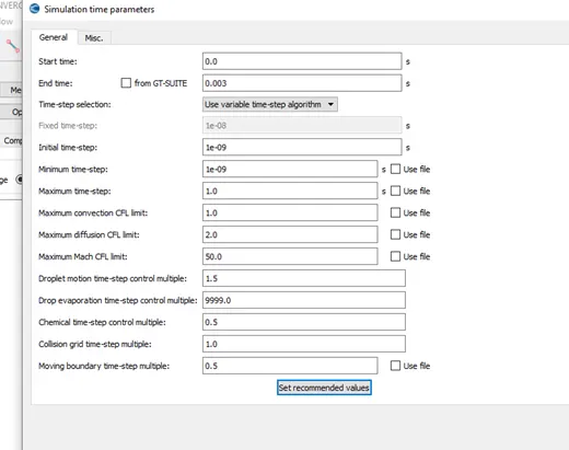
Simulation Parameters

Start time -0

End time:0.003 s

Initial time steps: 1e-09 s

Minimum Time Steps:1e-09 s

Maximum time steps: 1 s

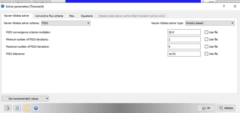
Slover parameters

Slover: Density Based Transient State Slover

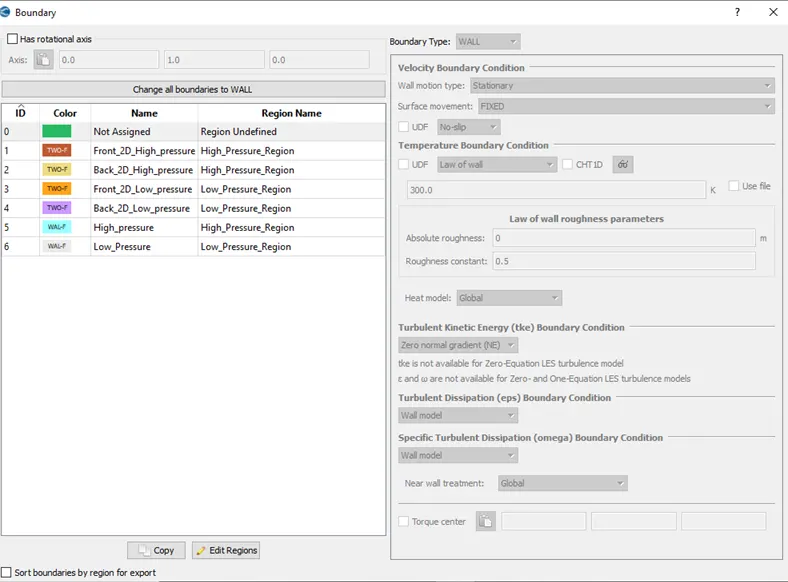
Boundary Condition

• High pressure Wall – slip

Temperature: 300 k

• Low pressure Wall – slip

Temperature: 300 k

• Front – 2D for both region
• Back-2 D for both region

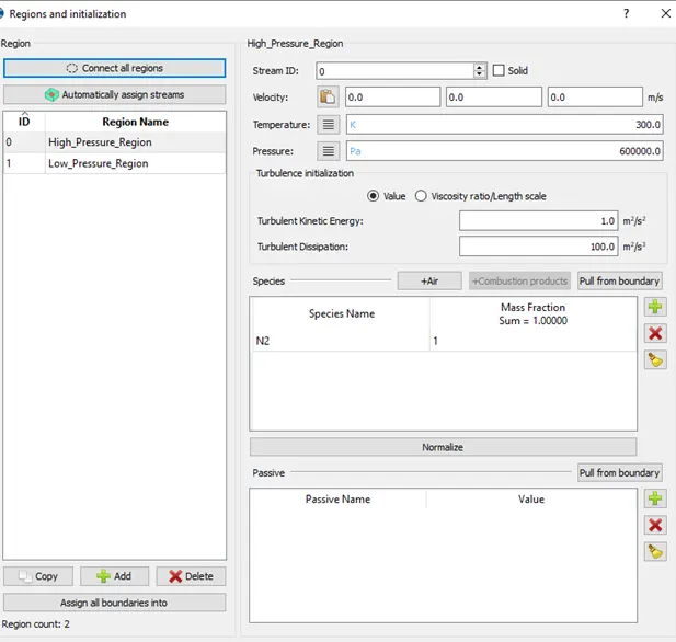
Region and initialization

High Pressure Region

• Region 0 – high pressur
• Pressure : 600000 pa
• Species N2 : 1

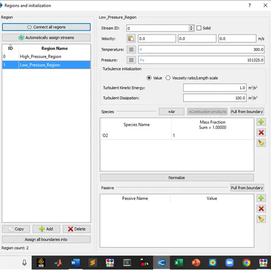
Low pressure region

• Region 1 – low pressure
• Pressure : 101325 pa
• Species O2 : 1

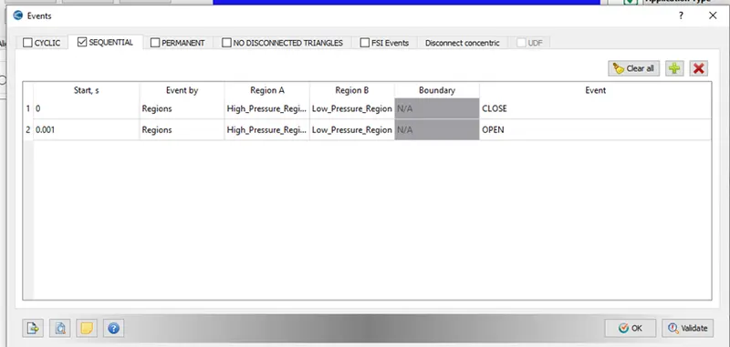
Events:

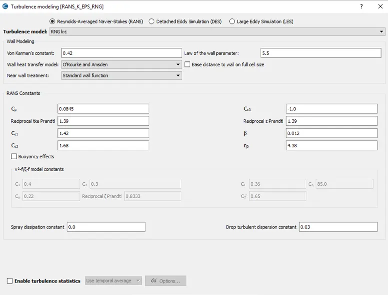
Turbulance Modelling

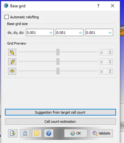
Base Grid

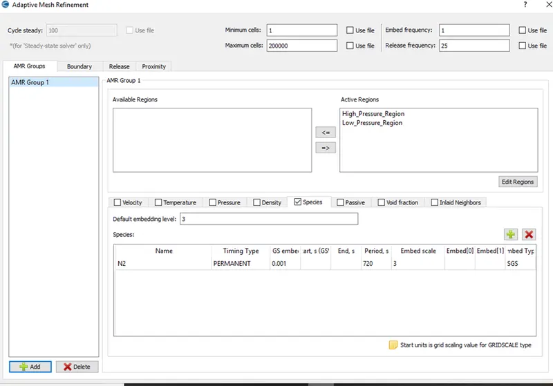
Adaptive Mesh Refinement

Final Validation: Check whether in any fault in your case set up if not proceed for simulation in Cygwin and then post process the results in Para view

Mesh

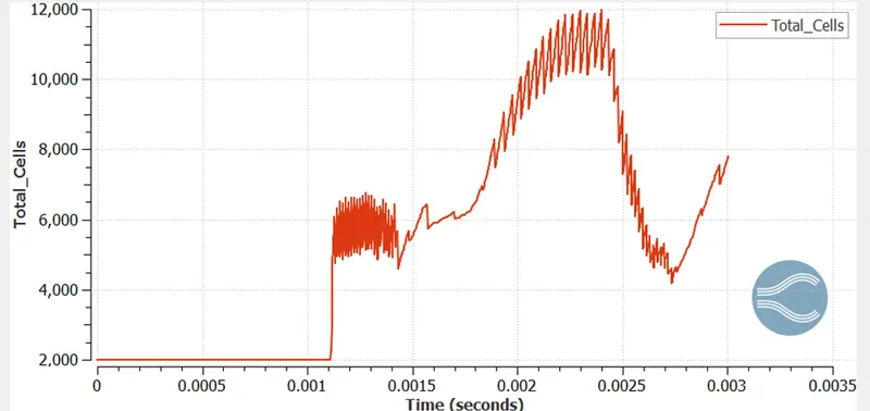
Total Cell Count:

Due to the Adaptive mesh refinement, it can be seen that the cells are changing with respect to time. We see that diaphragm has ruptured at 0.001 s the mesh size start changes. The refinement of cells is done according to SGS Criteria,

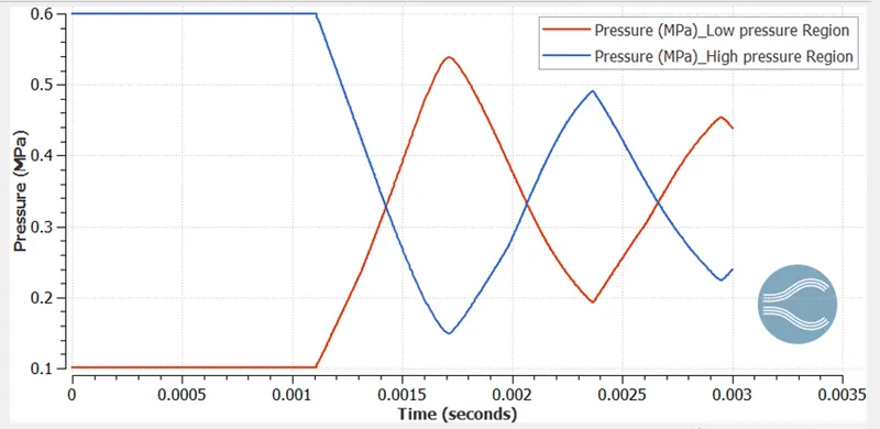
Pressure at Low pressure Region and high-pressure Region:

• Below graphs shows variation at high pressure region and low-pressure region.
• There is increase pressure in low pressure region and decreases pressure in High pressure region
• The pressure changes accordingly when the shock front is reflected back

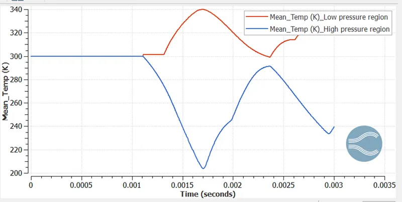
Mean Temperature at Low pressure Region and high-pressure Region

• Below graphs shows variation of mean temperature at high pressure region and low-pressure region.
• Temperature at low pressure region increases and Temperature at High pressure region decreases.
• Changes of temperature was seen with to & fro Movement of Shock

Animation Video:

1: Mass fraction of N2 across the tube: N2 from high pressure region produce shock and passes to the low pressure O2 region

Link:https://www.youtube.com/watch?v=2afDtPNuvKA

2.velocity Magnitude:

Link:https://www.youtube.com/watch?v=w4q1qIs0Xj4

Conclusion

• Simulation is run successfully for given shock tube problem
• There is increase pressure in low pressure region and decreases pressure in High pressure region
• The pressure changes accordingly when the shock front is reflected back
• We can easily conclude that cell count is function of time, AMR Phenomenon was studied