Week 7: Shock tube simulation project
Week 7: Shock Tube Simulation Project
Aim:
The main aim of the project is to set up a transient state simulation of shock tube with a diaphragm placed at the centre of the shock tube internally. To plot the pressure and temperature history in the entire domain. To plot the cell counts as a function of time and to explain the results. To display the mesh generation using PARAVIEW.
Introduction:
Shock Tube:
A Shock tube is a perfect example of an unsteady gas dynamic problem. The shock tube is a simple duct closed at both ends. A diaphragm divides this duct into two components called as the driver (high pressure) and the driven (low pressure) sections. These two sections are separated by a metal diaphragm. This shock tube is a device that is used to produce shock waves of varying strength in a controlled manner in the laboratory. It has several uses for scientific experimentation and mainly it is used in high enthalpy shock tunnel to study aerothermodynamics phenomenon of very high Mach number flows. When Mach number increases tremendously then there is significant increase in the stagnation temperature and pressures. Also they have various applications to interaction of shock waves with materials or structures that is relevant to blast waves because shock waves are also produced during an explosion.
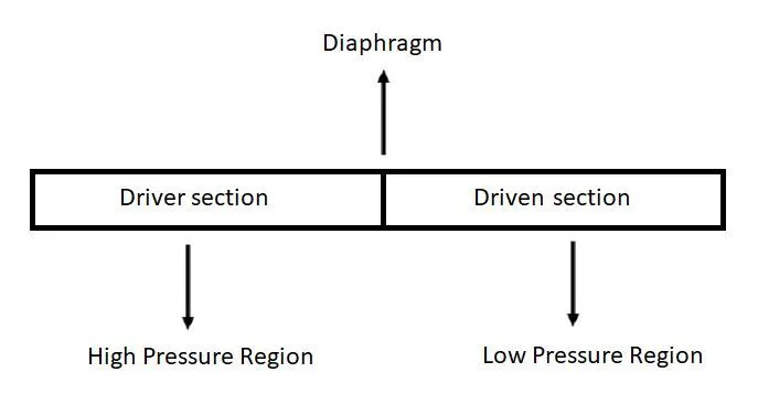
At the initial stage the pressure profile in the driver section have the high pressure and there is a sudden jump at the diaphragm section and low pressure in the driven section. At the initial stage the Mach number of both the sections remains to be zero as there is no motion taking place before the rupture of diaphragm.
When sufficiently high pressure is provided in the high pressure region, the diaphragm suddenly bursts. We can also use certain plungers to rupture the diaphragm at a specified pressure. The gases in the high pressure driver side and the low pressure driven side can be different depending upon the applications of the shock tube. The important parameters that is to be taken care for this shock tube is pressure, temperature and the speed of sound in both high and low pressure sections.
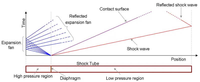
The moment the diaphragm ruptures within the shock tube, there is a large pressure difference between the two sections. The gas present inside is a compressible gas that results in compressible flow phenomenon and ultimately they lead to the formation of shocks. So as a consequence we have the shockwaves that travels within the driven section of the tube. Initially when the shock wave starts, there was a differentiation between the driver section and the driven section. So the shock wave progresses in the driven section that is in the lower pressure region but in the high pressure region an expansion waves are formed. Expansion waves are a series of waves that are more gradual and they are isentropic which reduces the pressure in the driver section.
Shock tube simulation:
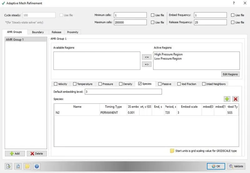
We are setting up 1D quasi transient shock tube simulation using converge studio and Paraview to post process the results. Pressure Difference of six bars is initially set between high and low pressure regions and 300 K as initial temperature in the domain. Nitrogen is used in the region of high pressure zone, therefore there is no need for enabling the reaction mechanism. Nitrogen based adaptive mesh refinement is used with 0.001 SGS embed and permanent type. By using the option 'Events', flow is allowed to take place between the two regions after 0.001 seconds. To make this happen we will be using 'Sequential' option in the event's tab.
Geometry Setup:
Import Geometry:
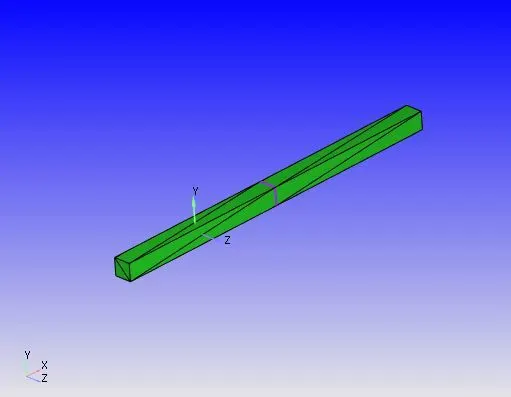
The STL file is imported in the converge studio software by using the following command.
File --> Import --> Import STL --> Select the STL file in the available location.
Diagnosis check:
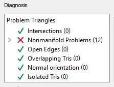
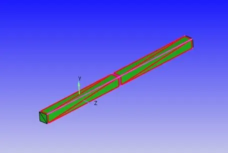
There are several intersections because of the diaphragm, which is created between the two parts in CAD modelling which is not required for the simulation. The non-manifold problem occurred due to the diaphragm vertices are shared by more than two triangles.
Deleting diaphragm:
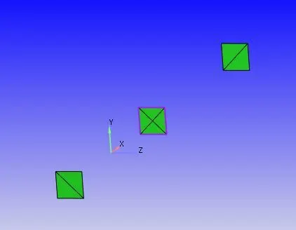
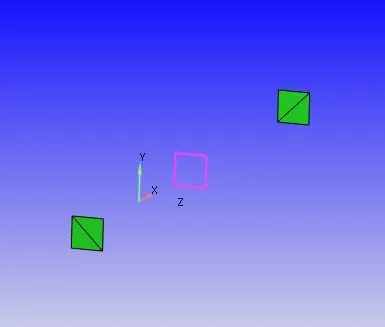
The diaphragm can be viewed by hiding the outer surface and the diaphragm is deleted by using the following command. Geometry --> Repair --> Delete --> Select the deletion type as Triangle --> Select the diaphragm section --> Click on Apply.
Normal Orientation:
The outer surface is redisplayed. Diagnosis check has been made again. In this check we could find error in normal orientation as the normals are facing outside. Since we are performing internal flow the normals must point inside the geometry. First we have to display the normal that is already prevailing. The normals pointing position is changed by using the following command. Geometry --> Transform --> Choose the selecting mode as any --> Select any one triangle --> Apply.
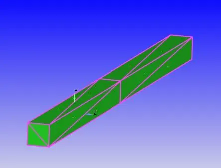
Another diagnosis check has been made, in which there we found no errors.
Assigning Boundaries:
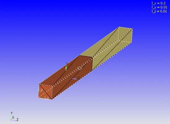
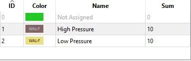
In converge every part of the geometry is assumed to be triangle. The group of triangles are assigned to form a boundary. The boundaries are formed by using the following command. Geometry --> Boundary --> Flag --> Add boundary --> Create two boundaries --> Select the particular triangles and allot them to one region --> Apply. In this project we have created two boundary regions (High pressure and Low Pressure).
Case Setup:
- The application type is fixed with time based.
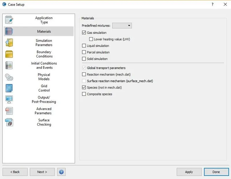
- Then click on Materials which is present in the right side of the window that is case setup tree and select the Predefined mixtures as Air and check the species option.
i) Materials:
- Click on the Gas simulation and Global Transport parameter and retain the same values.
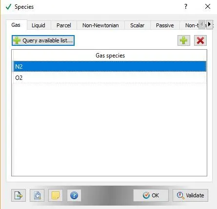
- Click on Species and then add O2 and N2.
ii) Simulation Parameters:
- Click on Run Parameters and under the solver tab choose the solver as Transient. Set the simulation mode to Full Hydrodynamic and the gas flow solver as compressible.
- Then under "Misc" tab uncheck the use shared memory boxes.
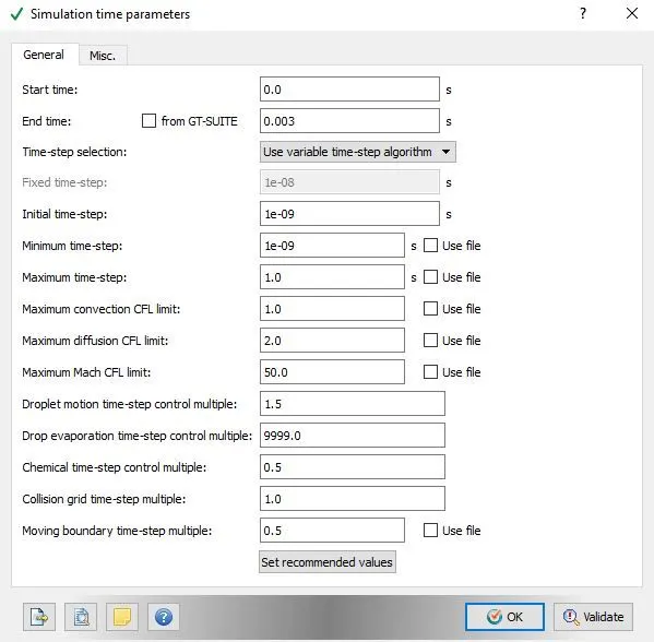
- Under Simulation time parameters set the start time as 0 s and the end time as 0.003 s and do the other following changes.
- Then under Solver Parameters retain the default settings.
iii) Initial Conditions and Events:
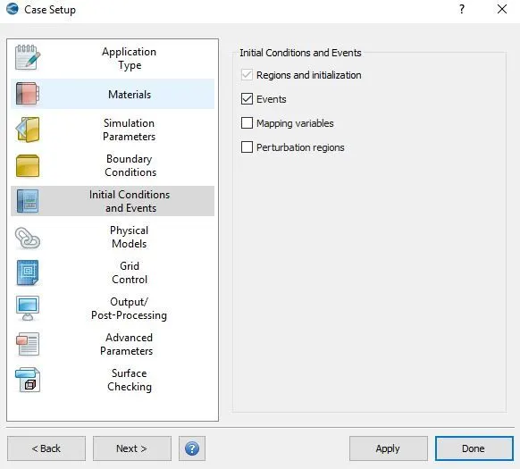
- Grouping the boundaries to form volumetric zones called region. This defines a volumetric region with initial conditions like initial pressure, initial temperature, velocity and species concentration.
- Enable Events option under Regions and initialisation tab.
iv) Regions and Initialisation:
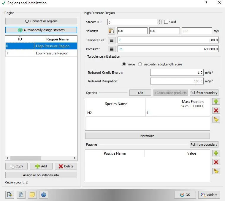
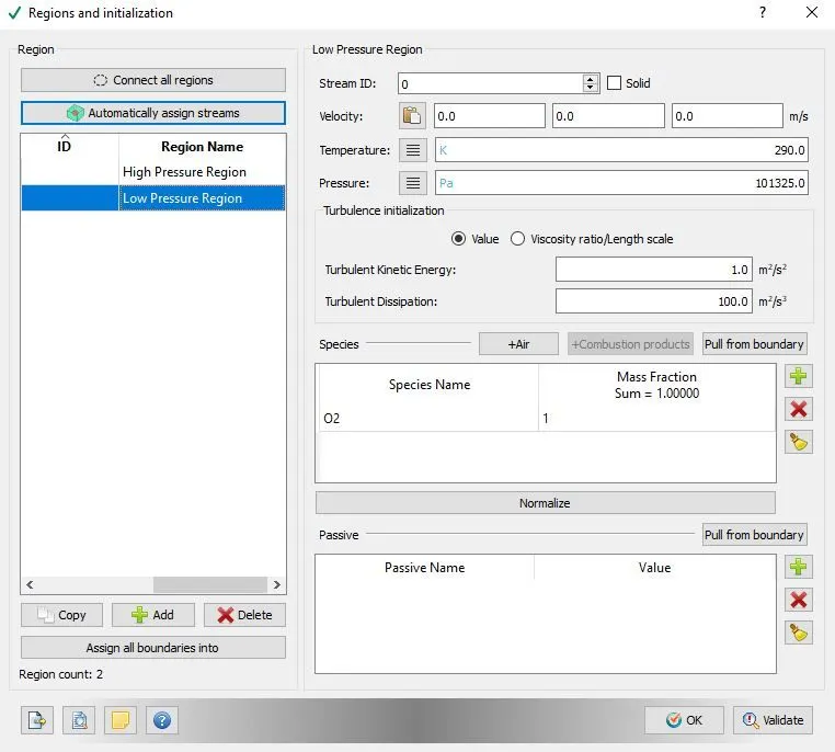
Under Regions and Initialisation, select add to create regions. Add 2 regions, naming High Pressure Region and Low Pressure Region.
High Pressure Region:
Low Pressure Region:
Events:
When 2 regions are in contact with each other with no boundary in-between them, it is necessary to use events. The events flag creates triangles in the place between the 2 regions called as disconnect triangles. Under Events tab do the following changes.
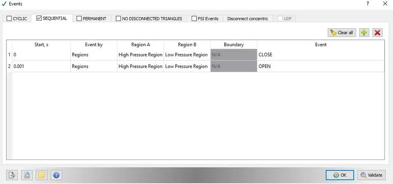
Events can be cyclic, permanent or sequential. Based on how the event should occur. In this case, the event can repeat itself in a sequence. Based on this setting, converge creates disconnected triangles. These triangles are temporarily created to simulate the event. Triangles are created for when there should be no interaction between the 2 regions and these triangles are deactivated when there is supposed to be an interaction between the 2 regions.
At the start, 2 regions are not in contact and for that event is set as given below:
- Start second: 0 sec
- Region A: High Pressure Region.
- Region B: Low Pressure Region.
- Event: Close.
After 0.001 seconds, to deactivate disconnected triangles and provide interaction between 2 regions the event is set as:
- Start second: 0.001 sec
- Region A: High Pressure Region.
- Region B: Low Pressure Region.
- Event: Open.
v) Boundary Conditions:
Boundary:
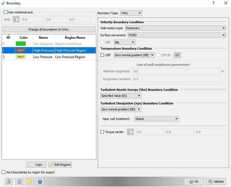
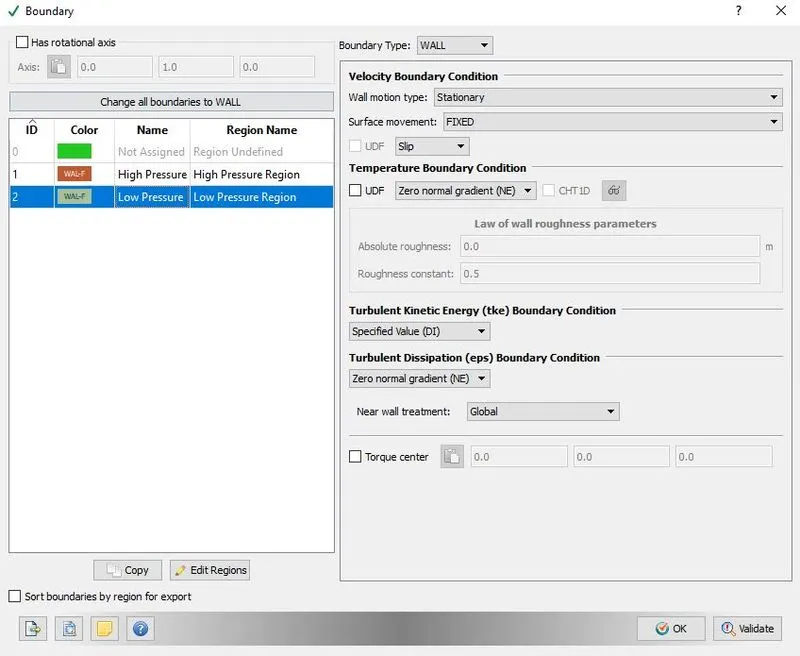
Under Boundary conditions assign the high and low pressure boundary with the following values.
High Pressure:
Boundary Type: WALL - Slip.
Velocity Boundary Condition:
Wall motion type: Stationary
Surface Movement: FIXED
Region: High Pressure Region.
Low Pressure:
Boundary Type: WALL - Slip.
Velocity Boundary Condition:
Wall motion type: Stationary
Surface Movement: FIXED
Region: Low Pressure Region.
vi) Physical Models:
Turbulence Modelling:
Then under the physical models check the turbulence modelling and set with Reynolds Averaged Navier-Stokes (RANS) and set the turbulence model with RNG K-epsilon.
vii) Grid Control:
Under grid control tab enable the Adaptive Mesh Refinement option.
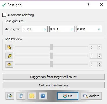
Then in the Grid Control parameter --> Base Grid --> Enter the size of the grid.
The size of the grid is assigned with 0.001 m.
Adaptive Mesh Refinement:
Adaptive Mesh Refinement is a method of adopting the accuracy of a solution within certain sensitive or turbulent regions of simulation, dynamically and during the time the solution is being calculated. When solutions are calculated numerically, they are often limited to pre-determined quantified grids as in the Cartesian plane which constitutes the computational grid or mesh.
viii) Output/Post-Processing:
Then under Output/Post-Processing --> Post Variable Selection --> Add the Mass fraction with O2 and N2
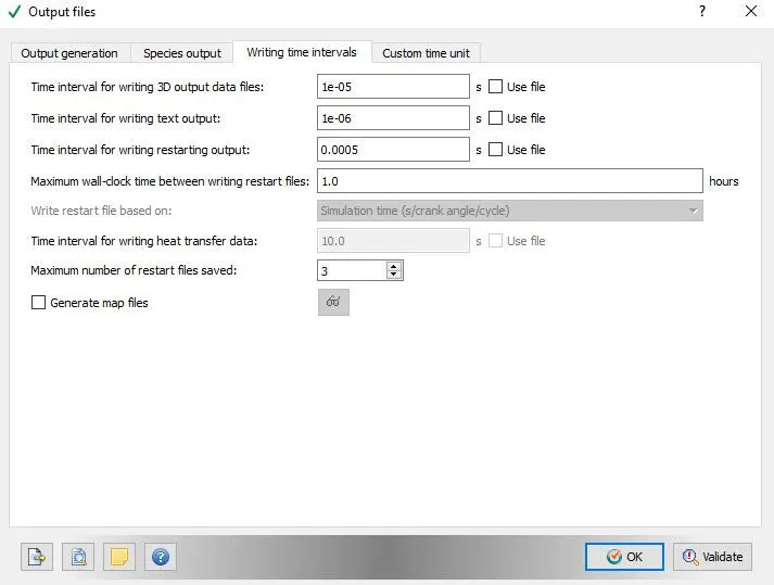
Then under the Output files --> Writing time intervals --> set the time interval for writing 3D output data files and time interval for writing restarting output.
Then use CYGWIN to execute the CFD solver.
Then with the help of Converge CFD the post converting the output files to Paraview format is done.
Paraview is used for Post processing the results.
Results:
Mesh:
Grid size: 0.001 m in dx, dy and dz.

The above mesh represents the mesh at time t=0. Since there are no flow movements at the initial stage, there is no adaptive mesh refinement phenomenon taking place.
Mesh with AMR:

Converge automatically generates an optimized Cartesian mesh at runtime and dynamically refines the mesh throughout the simulation using AMR. Converge kept monitoring the curvature of the fluid property provided in the AMR and the mesh refinement takes place when the property curvature variation between the consecutive grid is more than the defined SGS value. This is done to capture the flow properties in the shock flow region accurately. Due to AMR, the mesh is refined at the location where there are more changes in the slope of N2 mass fraction.
Mesh Animation:
From the mesh animation we could observe that the mesh refinement takes place at N2 - O2 interface and this mesh refinement keeps changing as the shock propagates back and forth.
Mass Fraction `N_2` Contour:
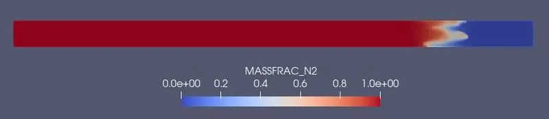
Since `N_2` is at high pressure, `O_2` cannot push `N_2`. So `O_2` cannot enter the high pressure region and it is completely filled with `N_2`. As the diaphragm breaks the high pressure region `N_2`pushes `O_2` the low pressure region and then the low pressure region reflects and pushes it towards `N_2`region. These shock waves keep moving back and forth as the waves have different pressures and due to which this occurs and after a while if the simulation is running for more time the pressure eventually settles and converges to a value.
Mass Fraction `N_2` Animation:
Mass Fraction `O_2` Contour:
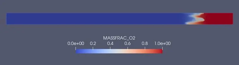
Since Oxygen is in low pressure region, it cannot push Nitrogen. So Oxygen cannot enter the high pressure region and it remains only at one end and resist mixing with Nitrogen initially.
Mass Fraction `O_2` Animation:
Pressure Contour:
The pressure field before the diaphragm's break is displayed. This shows the high pressure region in the left side and the low pressure region in the right side of the shock tube.
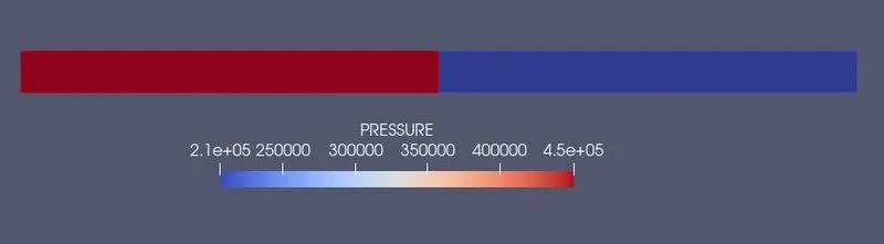
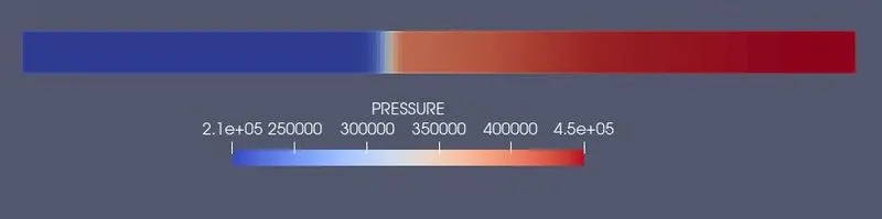
As the diaphragm is ruptured, the shock wave is generated and it enters the driven section by reaching the downstream end of the driven section. The shock wave produced is an oblique shock wave, where the static properties increases at shock occurrence i.e. pressure, density and temperature in the oxygen region increase. This also results in the expansion of nitrogen and hence the pressure decreases. The moment it hits the downstream end and gets reflected, their pressure values changes respectively and this flow pattern occurs till the shock intensity is decreased.
Pressure Animation:
Temperature Contour:
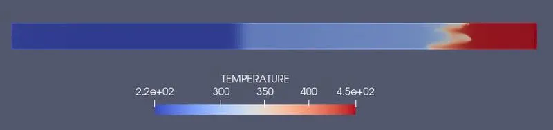
After 0.001 second, both the low pressure and high pressure sections are opened as the result of diaphragm rupture which leads to the expansion of high pressure nitrogen gas and it produces a shock wave which passes through the low pressure oxygen gas. The bursting diaphragm produces a series of pressure waves and they compress into a shock propagating the driven oxygen gas. These shock waves drastically increase the temperature in low pressure region and temperature of oxygen.
Temperature Animation:
Velocity Contour:
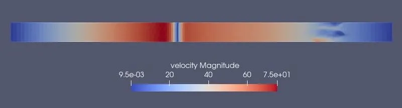
The velocity increases sharply as diaphragm burst and increases forth and decreases back and vice versa, such waves create shock patterns like diamond shock pattern is observed near the low pressure region.
Velocity Animation:
Pressure Plot:
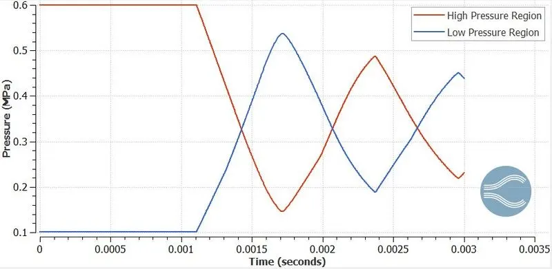
The high pressure region is at 0.6 MPa and from the plot, it is clearly visible that simulation never reaches that pressure. As soon as the diaphragm breaks at 0.001 seconds the pressure increases and the high pressure region pushed the low pressure region. Again the low pressure region pushes high pressure region and it is like pushing and dissolving until reflected wave occurs. Generation of a shock wave in the low pressure region leads to pressure rise and a slight drop in the plot is observed.
Temperature Plot:
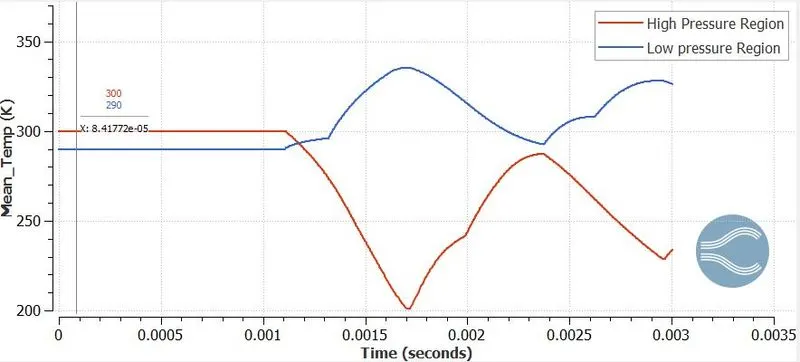
Initially the temperature throughout the shock tube is 300 K. After the break of diaphragm, regions are made open after 0.001 seconds. This leads to the expansion of high pressure nitrogen gas and it produces a shock wave which passes through the low pressure oxygen gas. The bursting diaphragm produces a series of pressure waves and they compress into a shock propagating through the driven oxygen gas. This shock wave increases the temperature in low pressure region and temperature of oxygen. The temperature in the low pressure region varies between 300 K and 340 K. The temperature in the high pressure region varies between 300 K and 200 K before attaining the steady state.
Cell Count Plot:
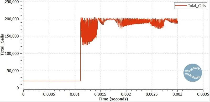
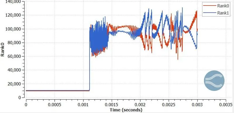
The cell count is changing due to the AMR (Adaptive Mesh Refinement) feature based on species that we have given. Under the events tab it was made in such a way that the diaphragm breaks at 0.001 seconds and as a result of that a sudden spike is observed. As the diaphragm opens the shock waves are produced. Nitrogen from the high pressure region enters into the low pressure region which will cause the mesh to become finer. This process i.e. the mesh becomes finer as a result of which the cell count increasing takes place until equilibrium is obtained, when both the gases are finished diffusing and an uniform pressure is obtained in the shock tube.
Conclusion:
- The transient state simulation of shock tube was performed successfully using the Converge CFD software and the Cygwin command prompt terminal.
- The shock tube is mainly used to study the properties of the fluid at an elevated temperature and pressure.
- The event option was enabled under the regions and initialisation parameter to connect the high pressure region and the low pressure region by a triangle which is called as a disconnected triangle.
- The burst of the diaphragm creates compression waves which propogate in the driven section and expansion waves transversing in the driver section. The shock wave when hits the wall it get refracted back and the mixing of the fluid occurs. The fluctuations in the pressure and temperature plots are observed during the mixing of two fluids. The generation of multiple shock waves inside the tube is beacause it doesn't have any outlet.
- From the pressure, velocity and temperature animations we could observe the formation of the shock waves and its behaviour.
- The cell count varies once the shock wave is created and this is because of AMR condition.