Week-7 : Converting a detailed engine model to a FRM model

Answer:-

                                                            Detailed Report On FRM

Aim:- To study the FRM Model.

Introduction:-

• Fast Running models are dynamic, which are designed to run fast.
• While high fidelity engine models are commonplace in the engine performance department, they are often too slow running to incorporated into system level models, where long transient events may be simulated. Also in this the simulation model must resond faster than real-time model.
• FRM are able to achieve fast run times by two ways:-
  1) By increasing the simulation time step size,
  2) By decreasing the no. of calculations per time step(iterations)
• These two means are often accomplished at the same time by lumping various flow volumes together which will reduce the total number of sub-volumes and also allow for a larger time step size by increasing the effective subvolume length.
• In addition to simplifying and combining flow volumes, there are additional solver options that can reduce the number of calculations per time step and, thus, further decrease the run time without changing the time step size.

Building a Fast Running Engine Model (FRM):-

• Launch GT-ISE and open the file SI_4cyl_GDI_Turbo-WOT.gtm from 'File' -> 'Examples' -> 'Engine_1D_Gas_Exchange_Combustion' -> 'Gasoline' -> 'SI_4cyl_GDI_Turbo'.

Remove Wastegate Controller:-

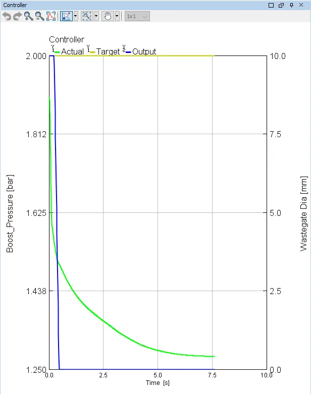
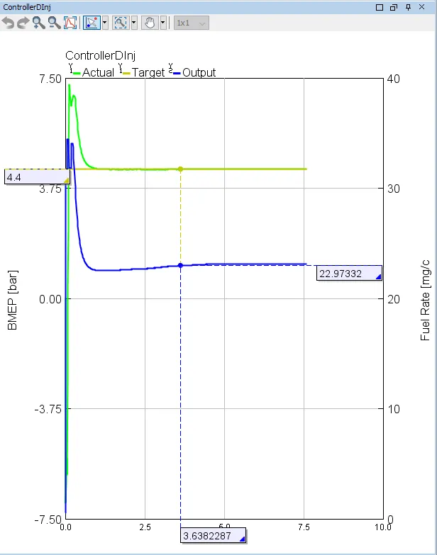
• In this example model, a wastegate controller was included to achieve the BMEP targets by adjusting the wastegate diameter.
• Before starting FRM reduction work, it is suggested to remove this controller.
• The reason is each step of the model reduction covered in the following needs to perform calibration,
  which aims to ensure the model still behaves similarly and achieve insignificant changes in the results after implementing the reductions.
• In order to make sure this calibration process is independent of any other factors but the desired calibration parameter, the best practice is to remove the controller at the beginning.
   

Launch FRM Tags:-

• Go to the Tools tab and click on 'FRM Tags'.

Launch the FRM Converter:-

• The GT-SUITE FRM Converter is a tool that will track the FRM Conversion process, organize all model files automatically within subdirectories,and provide result comparisons of key RLTs throughout the conversion process.
• With the high-fidelity engine model open in GT-ISE, go to the Tools tab and click on 'FRM Converter'.
• This will prompt you to create an FRM Conversion Project. It will validate the tagged subsystems and report if the validation is successful.
• Confirm that the correct model is specified in "Select the Baseline Detailed Model" per below, then click Next.
  In the "Accuracy Checking" dialog, select key RLTs to track the accuracy of the model as the conversion progresses.
• Optional Tolerances may be specified for which additional comparison plots will be generated, and the user will be warned if a particular RLT becomes outside of a given tolerance.
• Once the Accuracy RLTs and tolerances have been defined, click "Next (Begin First Step)" to begin the conversion process.

Step 1: Exhaust Manifold:-

• Simplifying the first subsystem of the model. It is most efficient to start by simplifying the subsystem that is currently restricting the time step.
• For high-fidelity models, this is almost always the exhaust manifold where the highest gas velocities occur, which in turn restricts the time step.
• Before we apply simplifications to the exhaust manifold, the Maximum Time Step limit of 1 crank angle degree will be removed.
• This is a default limit that is imposed when an EngCylinder component is in the model.
  If the Courant Condition allows for a larger time step (by monitoring gas velocity and subvolume length in all flow components), removing this limit will allow the time step to increase in size.
• Click "Collapse" at the top-left of the FRM Converter to collapse it into a smaller, more manageable dialog.
  Then, from the "Home" tab, click on "Run Setup" and go into the "FlowControl" folder, then double-click on the "ExplicitControl" green text within the "Time Step and Solution Control Object" attribute to edit the ExplicitControl reference object.
• Set "Maximum Time Step" to 720, then click "OK", and "OK" again to close Run Setup.
• Click "Expand" on the FRM Converter to expand the Model Reduction page. The Exhaust Manifold will now be simplified.
  Make sure that the "Apply Smart Calibration Settings" check box is selected.
• This option can be found below the simplify buttons. This setting prefills the attributes for the design optimizer used later for model calibration steps. If accuracy is of higher importance than run-time, choose the "Simplify for Accuracy" option.
• This will combine the Exhaust Ports/Runners together, and left separate from the manifold volumes.
  If a real-time capable model is required choose "Simplify for Speed". In this case the Ports, Runners, and Manifold volumes will be combined together at once.
• This will be performed in a later step, whereas accuracy will be the focus for now, so proceed by clicking on the “Simplify for Accuracy” button.
• Clicking on the "Simplify Manually” tab will allow to manually simplify geometry for parts that were not tagged or where a different combination of volumes is desired.

Step 2: Exhaust Pipes:-

• For the second step of model simplification, the exhaust pipes downstream of the turbine will be simplified.
• Name the step "Exhaust Pipes". Select "Exhaust Pipes 1" from the Tagged Subsystems list, as shown in the figure below.
• Click on "Simplify for Accuracy" and click "Yes" for the "Delete Part" dialog.
• Since the pipe at the outlet of the Turbine is rather short (70mm), this pipe will be combined with the Catalyst volumes into a single FlowSplit part, see the "Simplify Manual" tab for instructions.
• Select the "EP1_Pipe1-1" pipe along with the "EP1_PDrop1-1" FlowSplit and the OrificeConn between them, then right-click on the selection and launch the Combine Flow Volumes Wizard.
• Once in the Combine Flow Volumes wizard, keep "Combine flow volumes to Flowsplit" selected and click "Next" through the wizard until the last page, "Object Attribute Definition and Object Naming". Select "EP1_PDrop1-1" at the top of the dialog, then set the object name to "CAT".
• The Thermal tab shows that inputs are missing. We are dealing with it later, click "Finish". Hit Close in the "Combine Volume Wizard Report".
• Open up the "CAT-1" part and go to the Thermal tab. Select the radio button for "Imposed Wall Temperature". Edit (double Click) the "GasT" Reference Object.
• Use the value selector for the "Wireless Signal or RLT (X)" object value and replace "tav:catconn1" with "tav0:CAT-1” and click "OK".
• Close the object dialog for the "CAT-1" part as well.
• Lastly, we need to Open Case Setup and set the value of [DIA_Exhaust_Pipes_1_Step_2] to 40 mm. This is only an initial guess, and will be used to calibrate the Turbine Outlet Pressure.
• In the FRM Converter, click "Next (Set Calibration)". In the Calibration page, select all cases for calibration. In this step, this calibration uses optimizing each case independently.
• The model reduction has simplified the catalyst brick that consists of multiple pipes to a single flowsplit, the significant loss of complexity may make it difficult to find a single orifice diameter that can accurately capture the pressure losses across all operating conditions.
• However, this does not imply that this method applies to every user case of pressure drop calibration. Under "Configure calibration…", set the "Response RLT" to "Engine BMEP" like previous step, and set the lower and upper values of the "Range" at 35 and 45 mm, respectively.
• Run the calibration, and once it is finished, click "Next". At this step, it is suggested to not close the optimizer yet.
  In the Results page, click "Collapse" to check if the best designs from the optimization have been properly populated in Case Setup.
• If not, manually set up in the Case Setup. The orifice diameter for the five cases should be very close to that shown as below.

Step 3: Intake Manifold:-

• Name the step "Intake Manifold". Select Intake Manifold 1 from the Tagged Subsystems list. Click on "Simplify for Accuracy".
• Click "Yes" on the "Delete Part" dialog; this will be handled later. Collapse the FRM Converter to provide space to work in the model map.
• Minor modifications need to be made to the "Characteristic Length" and "Expansion Diameter" for the combined volume.
• Open the new "IM1_Plenum1-1" part and define the "Boundary Data" folder as shown below, with the values better representing the complete combined geometry.
• The characteristic length is defined as the distance that the flow entering the boundary will travel before crossing another boundary or impacting a surface.
• Boundary #1 represents the boundary between the flowsplit and "IM1_Pipe1-1".
• The fluid entering the flowsplit in this direction can travel all the way across the plenum before impacting a surface,
  so the characteristic length is equal to the length of the plenum.
• The other boundaries are adjacent to the runners, where backflow from the cylinder would travel across the diameter of the plenum before impacting the plenum wall, which is why they are given a characteristic length of 70mm.
• To resolve the "Delete Part" warning that was previously displayed, double-click on the EngineCrankTrain, go to the "RLT Norms" folder, and change the value of the attribute "Part Name for Manifold Volumetric Eff. Reference" to "IM1_Plenum1-1".
• Then, go into "Run Setup" -> "ConvergenceRLT" folder and change the first RLT Variable to "
  pav:IM1_Plenum1-1".
• To resolve the "Delete Part" warning that was previously displayed, double-click on the EngineCrankTrain, go to the "RLT Norms" folder,and change the value of the attribute "Part Name for Manifold Volumetric Eff. Reference" to "IM1_Plenum1-1".
  Then, go into "Run Setup" -> "ConvergenceRLT" folder and change the first RLT Variable to "pav:IM1_Plenum1-1".

Step 4: Compressor Outlet Pipes:-

• Name the step "Compressor Outlet Pipes". Select "Boost Pipes 1" from the Tagged Subsystems list. Click on "Simplify for Accuracy".
• Collapse the FRM Converter to provide space to work in the model map.
• Run the calibration, and once it is finished, click "Next". In the Results page, click "Run Model" to rerun the full set of Cases.
• After checking model results and assuring that they are satisfactory, click "Next (Begin Next Step)".

Step 5: Intake Pipes:-

• Name the step "Intake Pipes". Select "Intake Pipes 1" from the Tagged Subsystems list. Click on "Simplify for Accuracy".
• Collapse the FRM Converter to provide space to work in the model map.
• Run the calibration, and once it is finished, click "Next". In the Results page, click "Run Model" to rerun the full set of Cases.
• Check the model results and assure that they are satisfactory.
• If this runtime is satisfactory for a given application, the user may click "Finish" to exit out of the FRM Converter, where the final FRM will be saved.
• However, if additional run simulation speed is desired, further changes can be made to the model. Since each subsystem of the model has already been simplified, we will open the latest set of results in GT-POST to identify how additional simulation speed could be achieved.
• With the Results page of Step 5 still open, click on "View Results" in the Home tab of the GT-ISE toolbar. This will launch the results file (*.gdx) of Step 5 in GT-POST.
• In the GT-POST toolbar -> Home, click the "No Map" button . Then click on the "Report Tables" tab, expand the group "Flow Solution Numerics",
  Go back to GT-ISE and click "Next (Begin New Step)" in the FRM Converter.

Step 6: Additional Changes:-

• Name the step "Additional Changes". Select Exhaust Manifold 1 from the Tagged Subsystems list. Click on "Simplify for Speed".
• Run the calibration, and once it is finished, click "Next". In the Results page, click "Run Model" to rerun the full set of Cases.
• Check the model results and assure that they are satisfactory. Compared to previous five steps with “Simplify for Accuracy”, this step with “Simplify for Speed” ends up with accuracy check falls out of the specified accuracy range (red flags).
• However, the model now can be running around 1 xRT. In the FRM Converter, click "Next (Begin Next Step)".

Step 7: Cylinder Slaving:-

• The final simplification to the model will utilize the "Cylinder Slaving" capability of the EngCylinder component.
• Name the new step "Cylinder Slaving" and without tagging any subsystems, then collapse the FRM Converter to provide space to work in the model map.
• Right-click on any of the EngCylinder parts on the map and choose "Edit Parent Object". Go to the "Advanced" tab and for "Cylinder Slaving Option", select "slave-RT-full-v2017", then click OK. Now double-click on Cylinder-01, go to the "Advanced" tab, and set the Cylinder-01 override value of "Cylinder Slaving Option" to "master".
• Expand the FRM Converter and click "Next (Calibration)" to preprocess the model and continue to Calibration. Calibration will not be performed for this step, click "Next" and go to Case Setup to set the calibration target to be "ign" before click "Run Model" to run the full operating range with this latest modification.
• Note that the runtime is affected by the CPU, stored data, monitors as well as any other processes that are running while the simulation is progressing, so it is possible this final model may not run below 1 xRT on a given machine. To achieve faster runtime suppress storage in Output Setup -> Data_Storage like Instantaneous Plots, Time RLTs and if run local turn off monitors.

Step 8: Real-Time Solver:-

• This is the optional step.
• Click "Next (Begin Next Step)" in the FRM Converter. Name this new step "Real-Time Solver", then collapse the FRM Converter.
• To run with the real-time solver, the license type of the model must be changed. However, certain templates are not allowed with the real-time solver, and so they must first be removed from the model.

Model:-

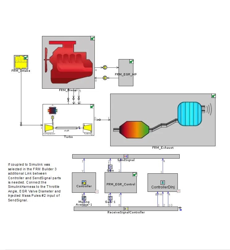
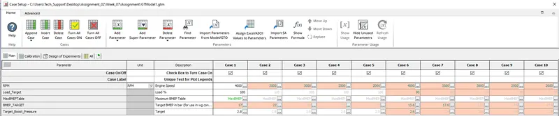
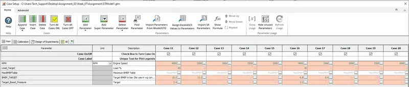
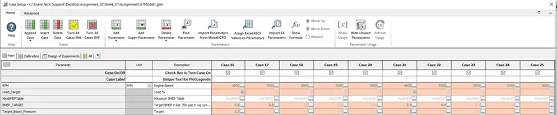
Results:-

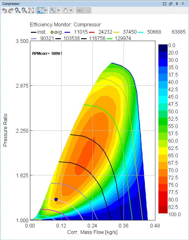
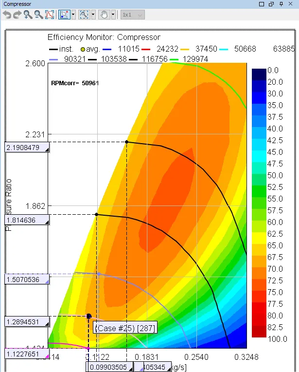
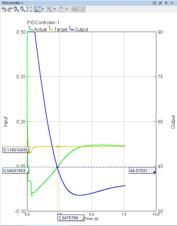
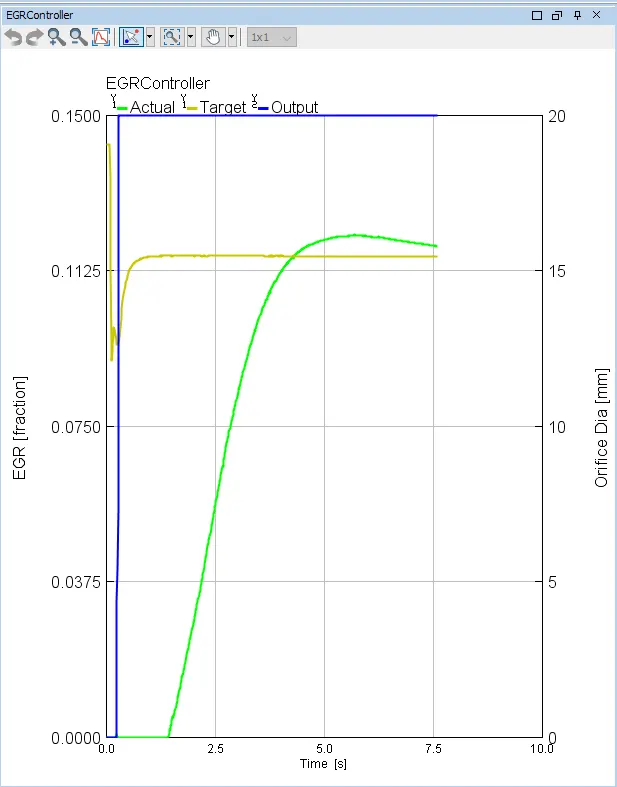
Conclusion:-

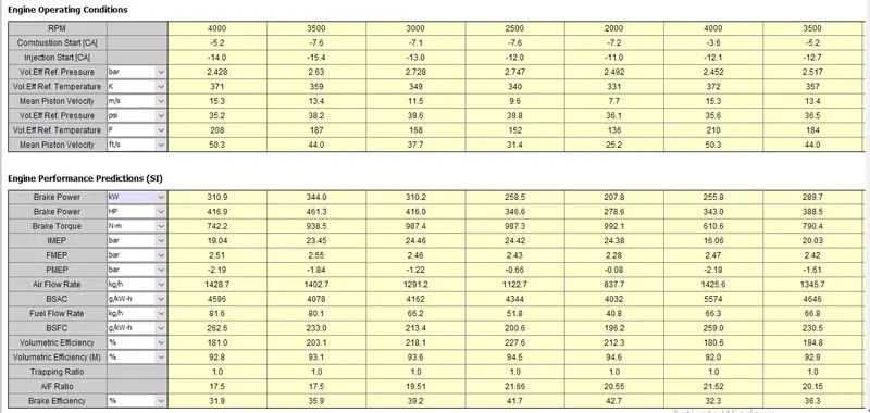
From the above results it is observed that the BMEP is having more impact on the FRM output, because when we change the value of BMEP from 17 bar  to 22 bar Power is increases from 416HP to 461HP & Torque increases from 742.2N.m to 938N.m