Challenge

Week-7 : Converting a detailed engine model to a FRM model

FRM models are created to run faster during simulation depending upon accuracy vs runtime requirement by the user. FRM can be created through two methods: 1) by creating a detailed map and convert into FRM model, 2) by providing engine specification & aspiration details and create "FRM developer"
Tutorial 9 model is given in the figure below:

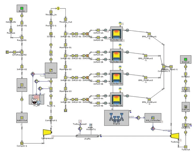
To create an FRM from a detailed model, GT-POST results are required to get an overview of potentially time-limiting parts so initially model will be run for all given cases. Simulation results are opened in the RLT contour map where pipe/Flow splits > Flow Control results are checked. In Flow Control, by courant time steps or Fraction of time spent gives an overview of limiting timestep for calculation.
After checking GT-POST, from FRM Tags a list of tags was created by tagging part on the map to identify subvolume and time-limiting parts of FRM conversion. FRM Tags can create new tags or remove created tags according to user requirements for FRM.

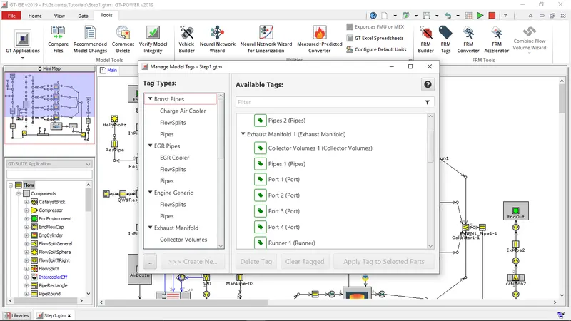
After creating tags, the next step is to FRM convert for that "FRM converter" in Tools Menu is used. when the FRM converter is selected entire model reloads in FRM from the saved model file. for the second time, a previously loaded model can be used. To proceed further it will require GT-POST Result file and confirmation to use that file for FRM converter.

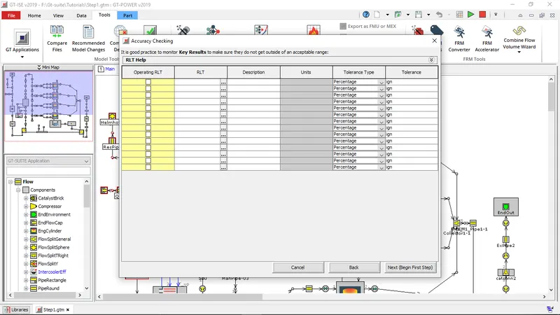
The next step is to select results that need to be monitor and can't be accepted outside tolerance. Click on "Next" following step1 screen showed. The first step always starts with "Exhaust manifold 1" because in the exhaust manifold maximum velocity occurs which restricts the time step.

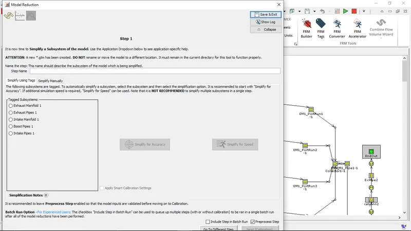
After selecting "Exhaust Manifold 1", From Run setup > Flow control, Maximum Time Step was set to "720" to allow time step to increase in courant condition. From here on FRM can be simplified into two targets, 1) For Accuracy and 2) For Speed. selecting any option will convert the model into the real-time capable model for the selected target. In the case of, non-tagged parts, a manual selection option is available. After simplifying the model, Discretization length and Temperature parameters are modified for the selected simplification method. The next step is to calibrate the model for which model will be preprocessed.
After preprocessing given "Calibration" screen will be open.

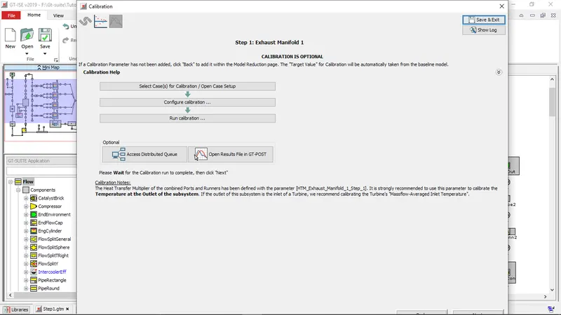
In shown screen, "Select case for calibration" will provide options to select cases to calibrate in simulation. "Configure Calibration" will open Design Optimizer to set target value and dependent parameters & limits. Set value and close the design optimizer. Next run calibration.

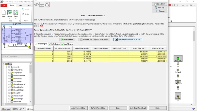
After calibration is complete, all turned-off cases will be turned ON and the optimizer will be set off. Next, "RunModel" and open "Populate Accuracy RLT Tables below" after the simulation is done.
Click "Finish" if the FRM target is achieved or click "Next" to begin calibration of other systems. The next steps are the same as the "Exhaust manifold" calibration steps.

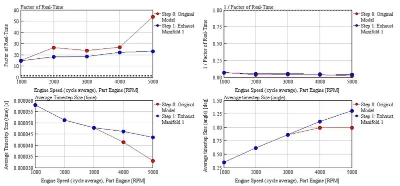
Step 2 - modeling was done on the "Exhaust pipe" for the Turbine to optimize pressure. Step2 - FRM results are shown in the figure below.

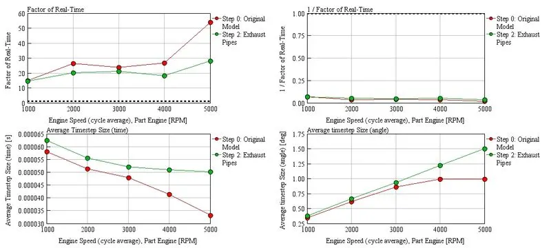
The following steps are similar to step 1 for simplifying the model for the compressor.

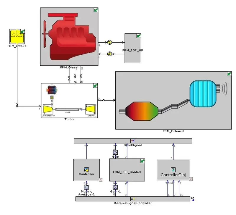
Figure - FRM model

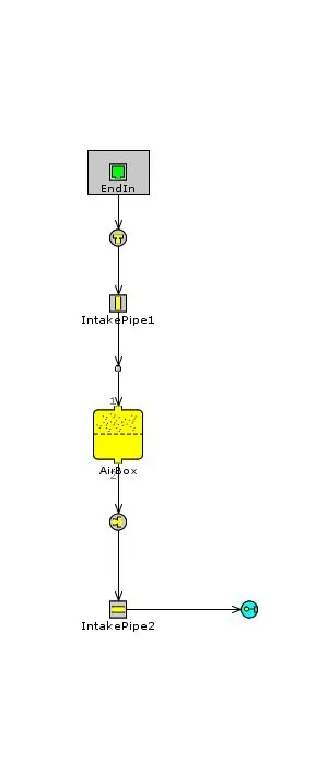
Figure - FRM Intake part

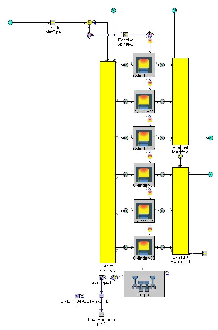
Figure - FRM cylinder & Crank train part

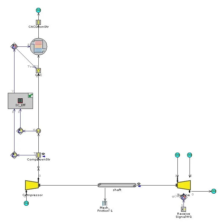
Figure - FRM Turbo part

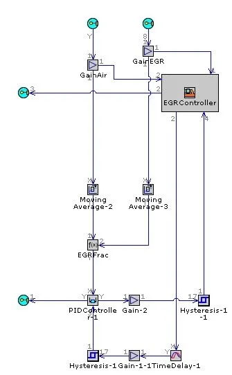
Figure - FRM EGR control part

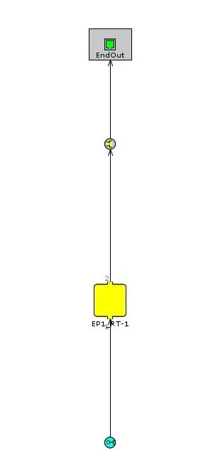
Figure - FRM Exhaust part

Result of all case run
For 3500 RPM, the engine all load conditions have the best performance compared to all other speeds & load conditions. In terms of Brake power, the highest power 329.9kW achieved at 3500 RPM for 100% load, the Highest brake torque at 990.47 Nm at 2500rpm & 100% load, and in terms of the highest efficiency, the highest is 43% at 2000 RPM & 1000% load.
A/F ratio ranged between 17.5 to 52.5 is unacceptable for above 25, the highest value A/F ratio is achieved at low speed and low load conditions.
For emission, it observed that NOx production is low at low load conditions but at higher load conditions, high speed has low NOx emission. CO2 emission in ppm is higher under 3500 RPM speed. For CO emission it is observed it is increased drastically after 3500 RPM under full load conditions. HC emission is very limited and no soot emission was found for any of the simulation conditions.

Ship work like this
in your own course.