Week 7 - CHT Analysis on a Graphics card

Aim: Perform a steady-state conjugate heat transfer analysis on model of graphics card

Objective:

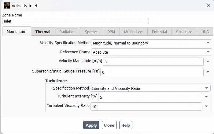
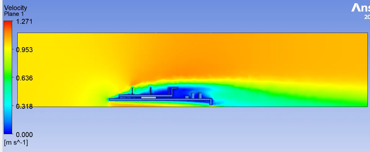
• Run the simulation by varying the velocity fron 1m/sec to 5 m/sec for at least 3 velocities and discuss the reults.
• Find out the maximum temperature and heat transfer coefficient attained by the processor.
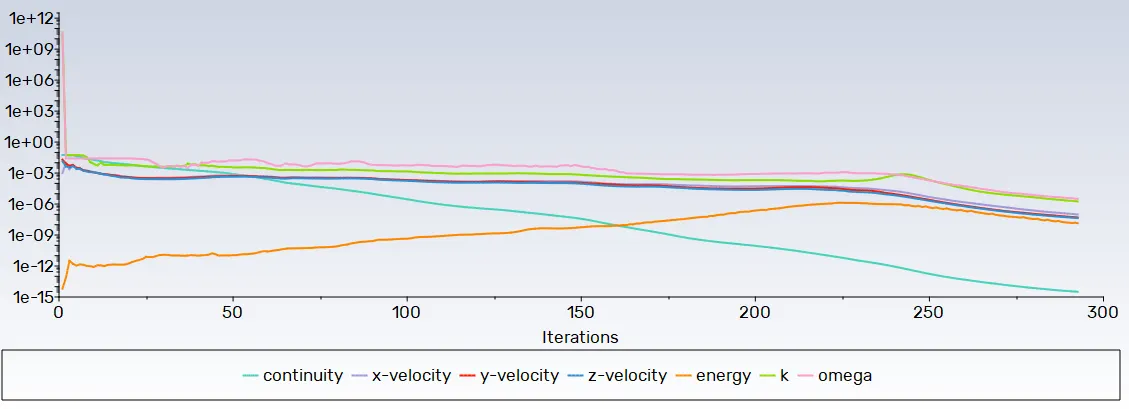
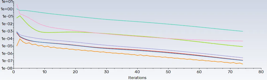
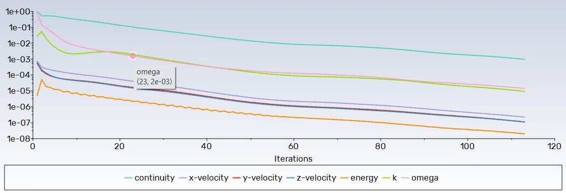
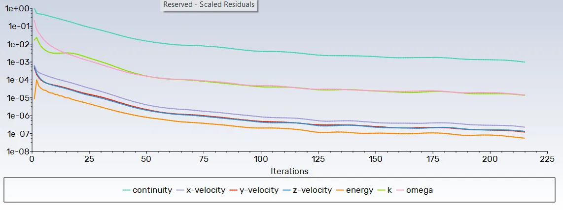
• prove that simulation has achived convergance with appropriate images and plots.
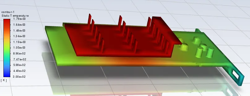
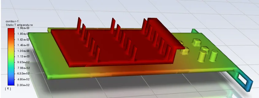
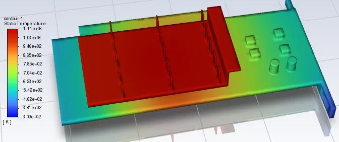
• Identify potential hotspots on the model.

Theory:

Conjugate heat transfer:

The conjugate heat transfer(CHT) analysis type allows for the simulation of heat transfer between solids and fluids domains by exchanging thermal energy at the interfaces between them. Typical applications of this analysis type exist as, but are not limited to, the simulation of heat exchangers, cooling of electronic equipment and general-purpose cooling and heating systems.

Examples:

HVAC, Heat exchanger, Tank, Internal combustion Engine, Heat Sink, Boiler,Reactor,Heat pipe, Turbocharger.

Heat Transfer in a Solid- Conduction: Diffusion of heat due to temperature gradients in solids. A measure of amount of conduction for a given gradient is heat conductivity. Conduction is described by Fourier's law defining the conductive heat flux, q,proportional to the temperature gradient.

Heat Transfer in Fluid- Convection: When heat is carried away by moving fluid. The flow can either be caused by external influence, forced convention or by buoyancy forces, natural convention.

Due to the fluid motion, there are three contributions to the heat transfer:

• Conventive contribution: Depending on the properties of fluid and its region of flow, the domination of conduction and convenction varies.
• Viscous effects: Due to the fluid flow, the viscosity creates heat. This effect is often neglected due to its negligible vale but should be taken into account for high velocity cases.
• Density effects: When the density becomes related to the temperature , the domain will have different densites at different location based on the temperature distribution. This variation in density can cause the compression which in-turn generates the heat.

The contemporary conjugate covrntion heat transfer model was developed after computer came into wide use in order to substitute the empirical relationof propotionality of heat flux to temperature differnce with heat transfer coeffcient which was the only tool in theoretical heat convenction since the time of Newton.This model, based on strictly mathematically stated problem, desribes the heat transfer between a body and fluid flowing over or inside it as a result of thr interaction of two objects. The physical processes and solutions of the governing equations are considered seperately for each object in two subdomains. Matching conditions for these solutions at the interface provide the distributions of temperature and heat flux along the body-flow interface, eliminating the nreed for a heat transfer coefficient. Moreover, it may be calculated using these data.

Application:

Starting from simple examples in the 1960s, the conjugate heat transfer methods have become a more powerful tool for modellinng and investigating natural phenomena and engineering systems in different areas ranging from aerospace and nuclear reactors to thermal goods treatment and food processing, from complex procedures in medicine to atmosphere/ocean thermal interaction in meteorology, and from relatively simple units to multistage, nonlinear processes. A detailed review of more than 100 examples of conjugate modelling selected from a list of 200 early and modern publication shows that conjugate methods are now used extensively in wide range of applications. That also is confirmed by numerous results published after this book appearence(2009) that one may see, for example, at the Web of Science.The applications in specific areas of conjugate heat transfer at periodic boundary conditions and exchanger ducts are considered in two recent books.

Geometry set-up:

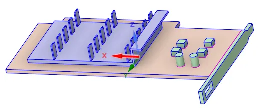
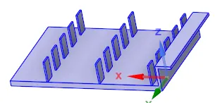
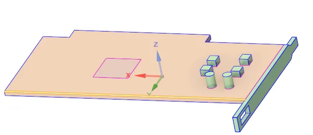
• Use Spaceclaim to edit the geometry of the downloaded model of the graphics card and to create enclosure.
• Click on share prep to view any edges in interference so that conformal mesh can be achived between different components.
• Share topology has to be enable between the different components so that necessry innformation can be shared between different zones of mesh.

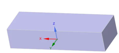
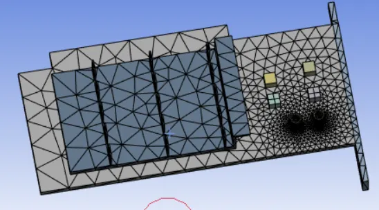
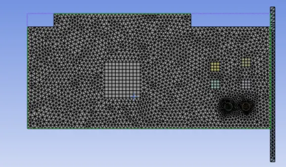
Graphics card

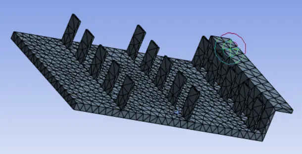
Fins

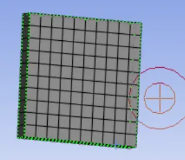
Processor

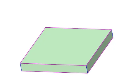
Base

 Mesh:

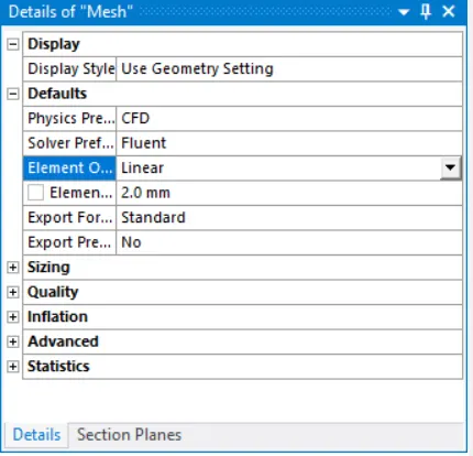
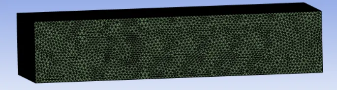
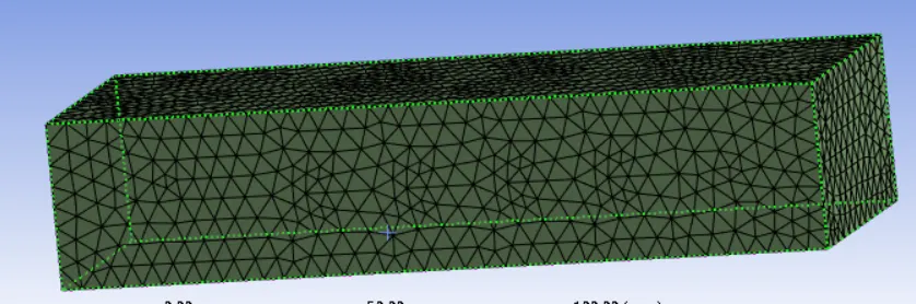
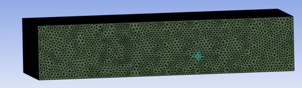
• Open the mesh set up using the face and body option to select the body to create the names to the each surface.
• After to create the basic mesh and refine the mesh based on the results of base level mesh.

Fluent setup:

Setting up the physics:

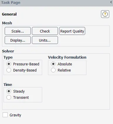
Setting up the physics for CHT analysis on graphics card in ANSYS fluent.

For this case we are using pressure-base steady state solver,Velocity formulation-Absolute.

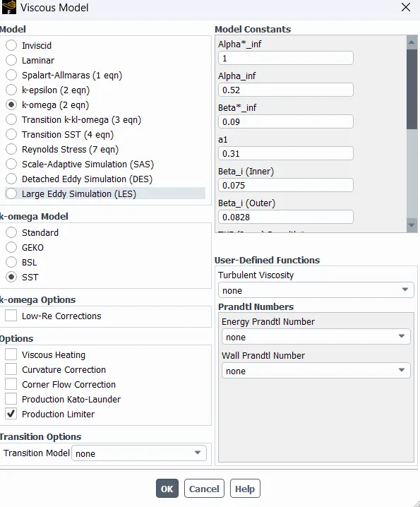
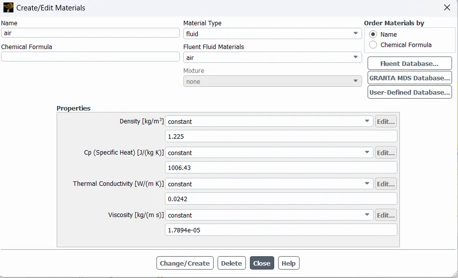
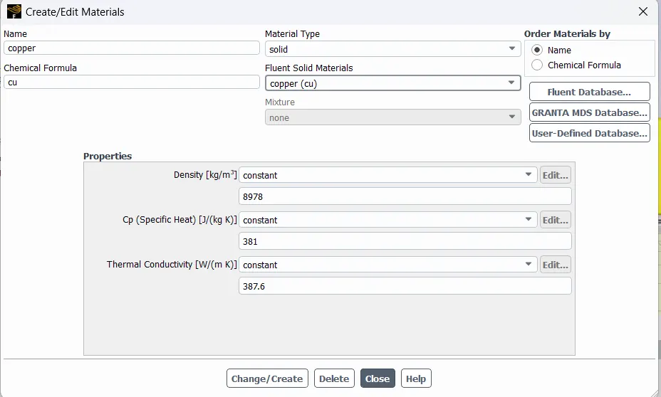
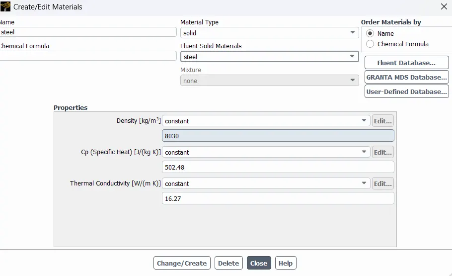
Setting up the source terms:

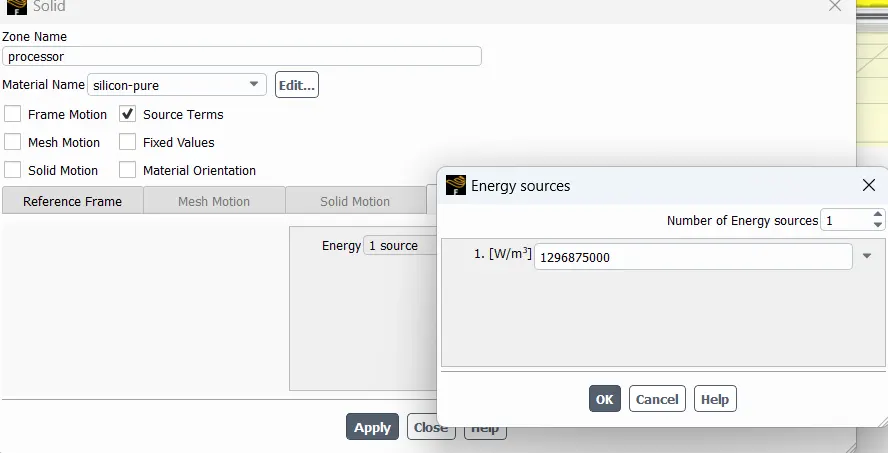
• For this case we consider that, our processor is a source terms and it generating heat.
• So, for setting up the source term go to Zones-cellzones-and click on the processor for editing which is in the solid.
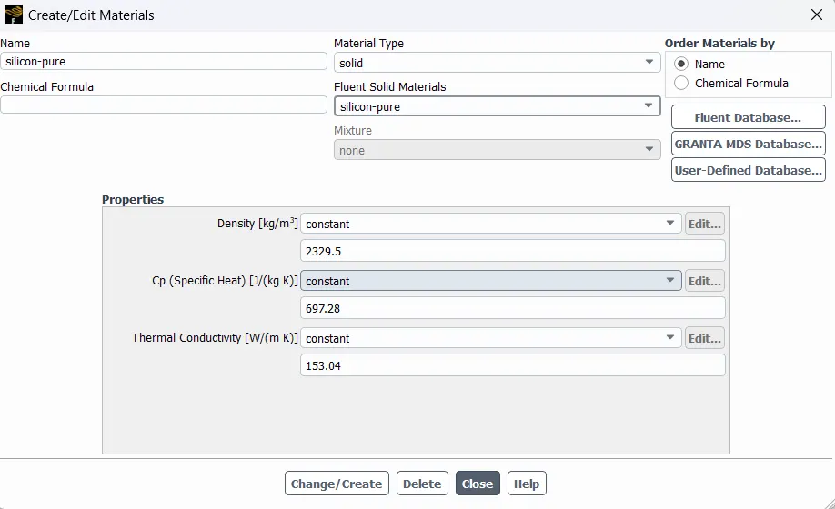
• After that select the material to gold and clik on souce terms to enable it and set the energy source to 1.

Calculate for the energy source:

Let the processor consume 83W of power to work.

Dimension of the processor=8*8*1 mm^3

So, Energy produced by the processor is 1296875000 w/m^3.

 

 

 

 Results:

Case1:

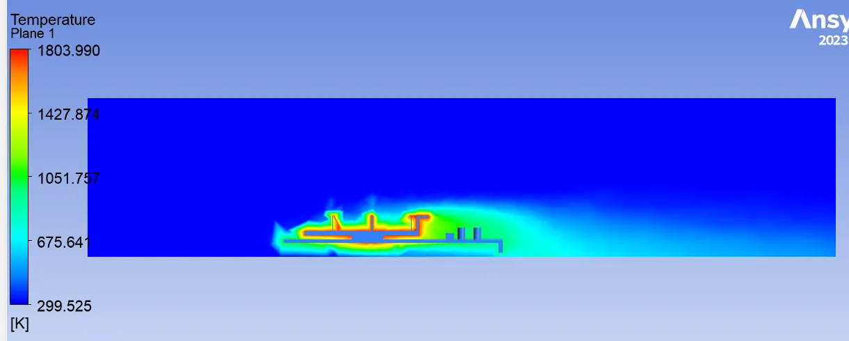
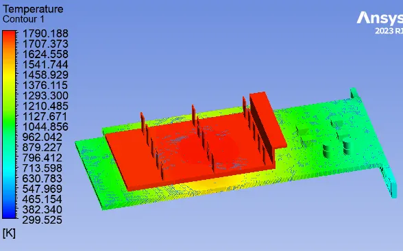
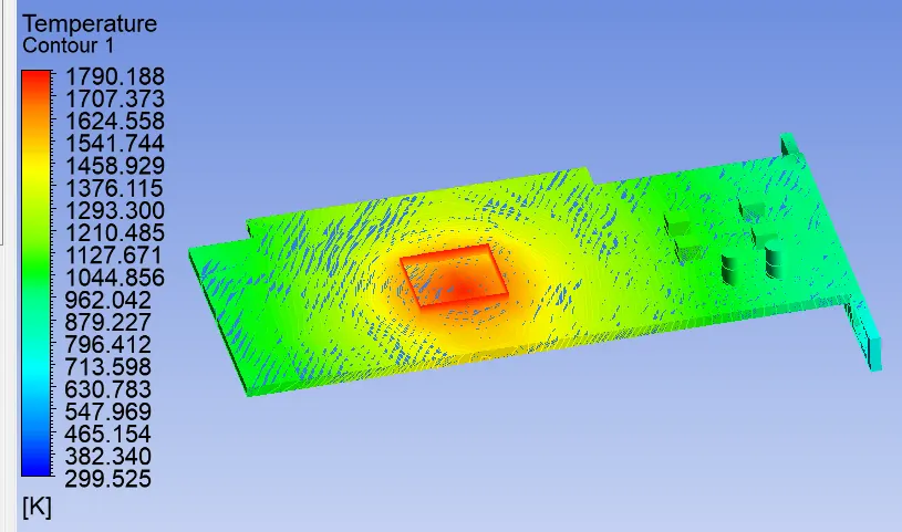
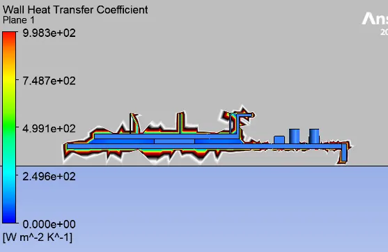
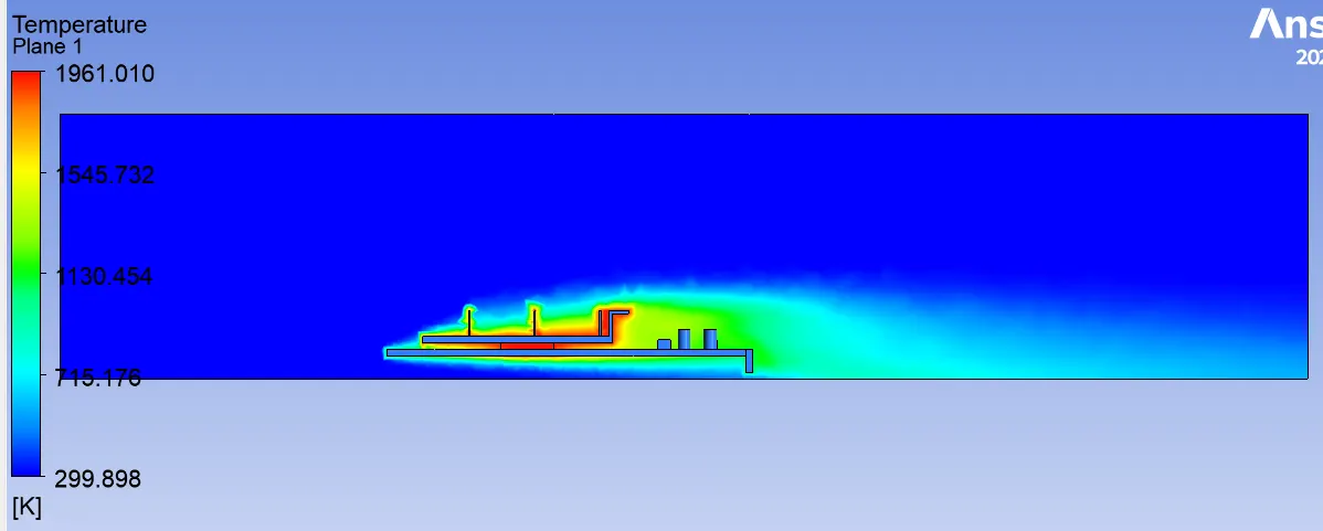
• Foe base mesh, velocity =1m/s, no.of iteration=500, step size=1

Residuals:

 

 

 

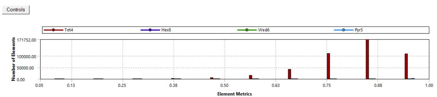
Case2:Refine mesh

We used element size=2mm

Body size of elements=0.8mm for base and capture curve is turned on.

Body size of elements=0.6 mm for fins and capture curve is turned on.

Body size of elements=0.2 mm for fins and capture curve is turned on.

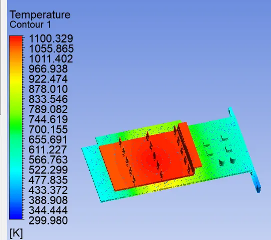
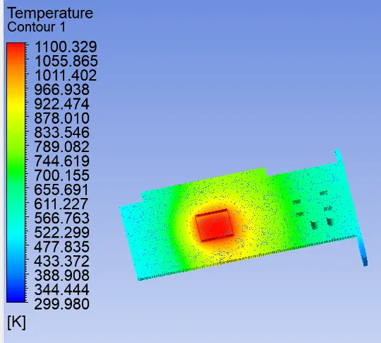
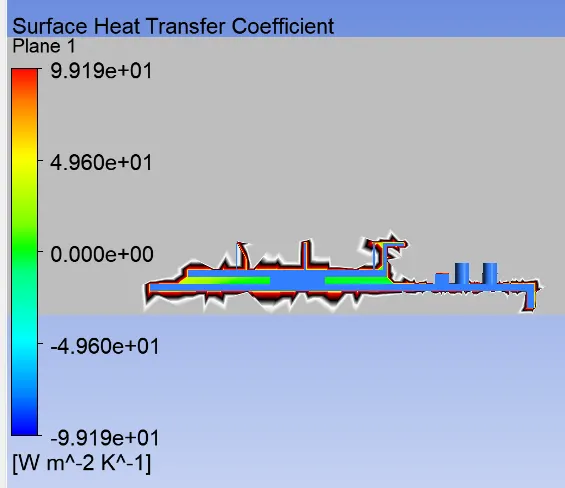
Case:3

velocity=3mm

 

 

 

 

 

 

 Case:4

Velocity=5mm

 

 

 

 

 

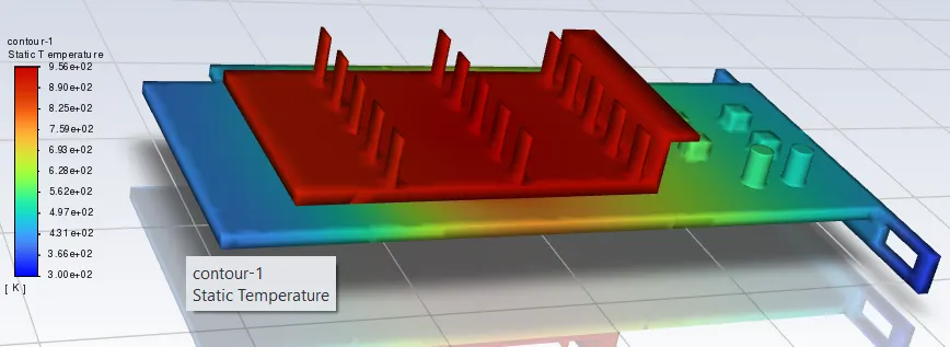
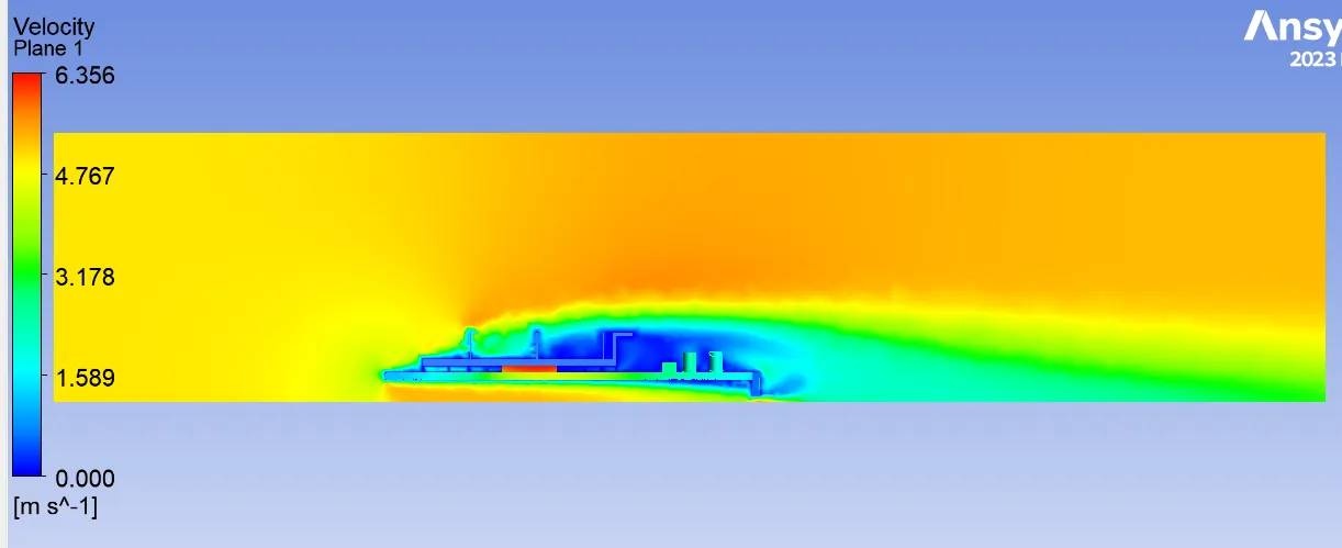
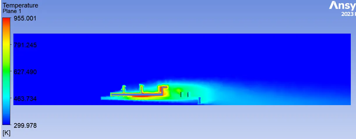
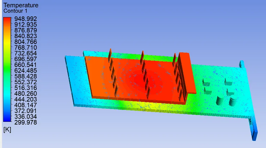
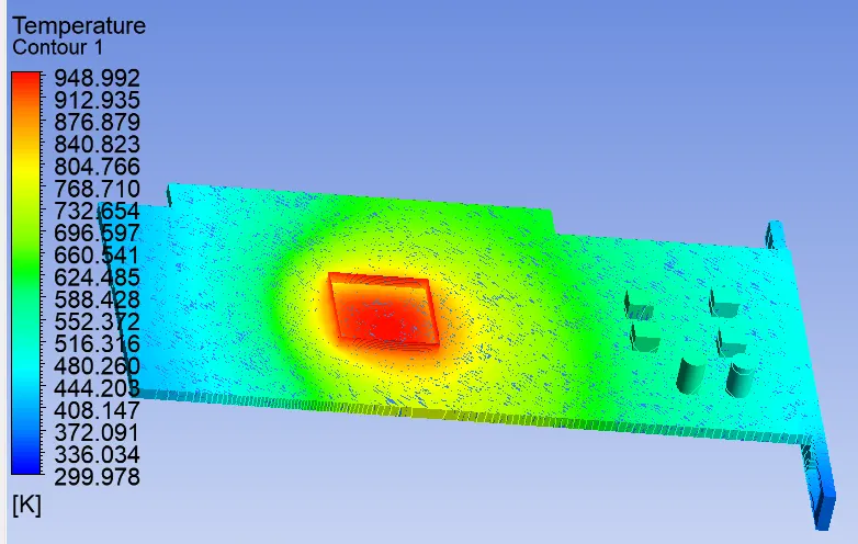
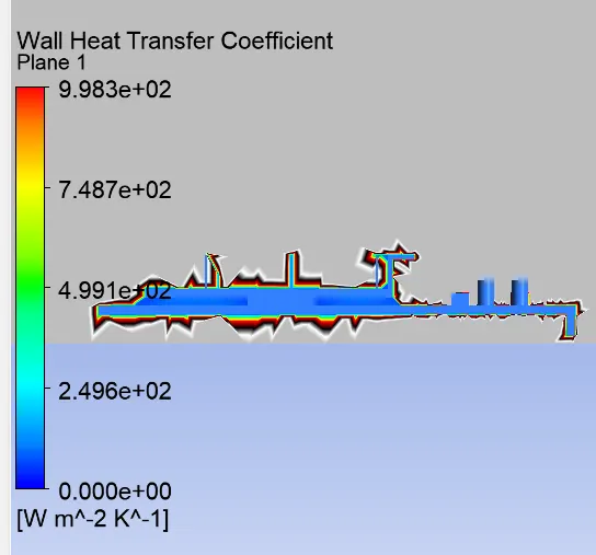
                         Velocity              temperature                     Wall Heat transfer Coefficient

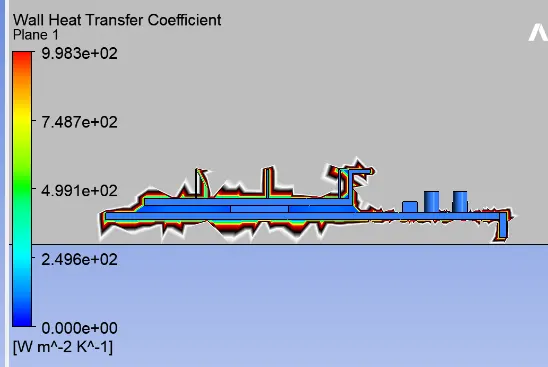
Case1                 1m/s                 1790.188                            9.983e+02

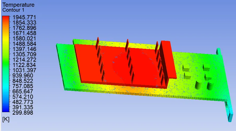
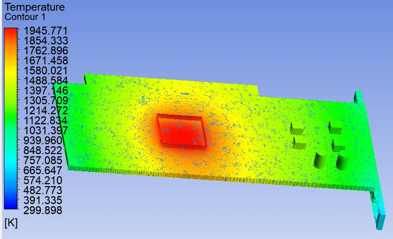
Case2                 1m/s                  1945.771                           9.983e+02

Case3                 3m/s                  1100.329                           9.919e+02

Case4                 5m/s                  948.992                             9.983e+02

 

Conclusion:

A converged solution for the given sets of input was observed on the basis of repetitive plots in rasidual plots. The processor acted as a source of heat input and thus one of the hotspots for such study.

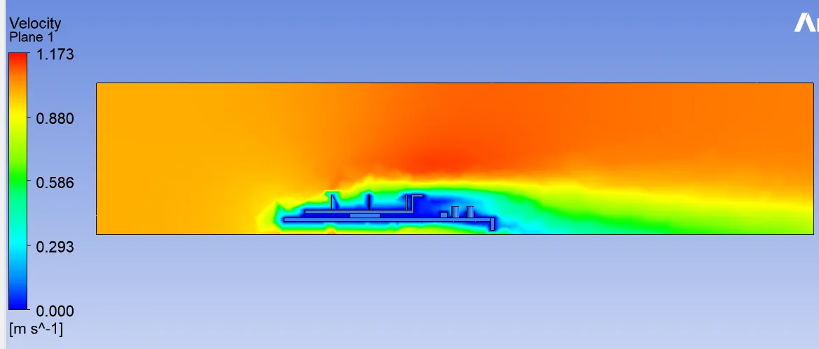
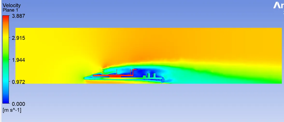
With an increase in velocity, we saw a considerable drop in temperature and a substantial rise in heat transfer coefficient which shows that high-velocity air can be an effective mode of heat dissipation in graphics card.

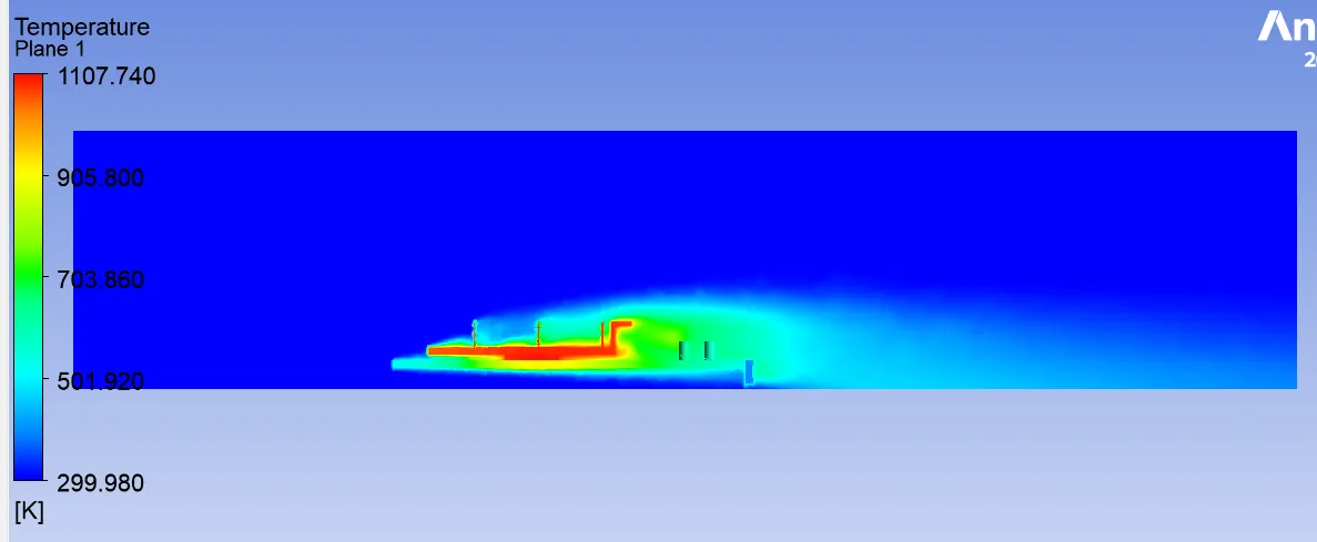
From the temperature distriution, we can see hotspots in fins and base near the surface that is in contact with the processor. Based on the thermal conductivity of the material this temperature is distributed accordingly amongest the component. We see few high-temperature zones on fin away from processor depicting their high susceptibility to heat due to their geometry.

Also, the differnce in baseline mesh and refine mesh is considerable and thus we can conclude that more refined mesh provides a better solution and can be used in optimizing the design for such applications.From the residual plot, the change in the gradient is very high which we can conclude that the solution has converged.

The high-temperature regions are found at the center of the fins, base, and processor walls. With further iterations, the temperature is distributed to other regions in the graphics card in the direction of the inlet airflow. Conduction occurs where there is a contact region between the solids in this case it is between processor and base and processor and fins. With the increase in the airflow velocity, the heat removal process by convection is faster.