Week 7 - CHT Analysis on a Graphics card

AIM:

To perform a conjugate heat transfer analysis on a graphics card and to obtain the following result:

1. To find out the velocity of the cooling air at which the there is a maximum heat transfer coefficient (h.t.c)
2. To find out the maximum temperature attained by the processor in every cases simulations performed
3. To identify the potential hotspots within the graphics card.

Theory:

Conduction through solids, forced and free convection in gases and fluids, and thermal radiation are just a few of the pertinent solid and fluid heat transfer processes that can be virtually solved using computational fluid dynamics (CFD) and, more specifically, conjugate heat transfer (CHT) analysis to predict heat transfer with accuracy.Since the wall heat transfer coefficients and their local fluctuations on surfaces are calculated directly within the model rather than relying on streamlined empirical computations, the CHT approach in particular has significant advantages over the Finite Element thermal analysis.Therefore, applications where heat transfer is either non-uniform or challenging to quantify empirically can benefit from the CHT technique.

The rendering of an image for a monitor is the responsibility of the graphics card.As a result, during this process, the processor of the graphics card heats up and produces a lot of heat. To ensure that the graphics card performs at its best without overheating, it needs to be cooled down using the right method.In most situations, a fan is utilised to circulate cool air over the graphics card. This causes forced convection heat transfer, in which heat is transferred to the incoming air and the component cools.Velcoity is therefore crucial to the forced convection heat transfer process.Therefore, using this simulation, we will ascertain the speed at which effective cooling occurs.

1.GEOMETRY:

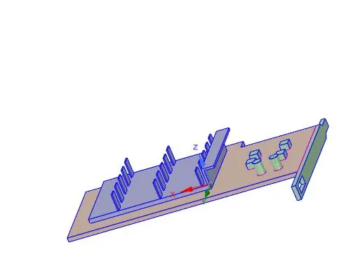
The geometry above is of the graphics card that were are simulating.Since the flow is taking place over the graphics card,an enclosure is provided and it is treated as the fial geometry for the simulation of the flow.

2.MESHING:

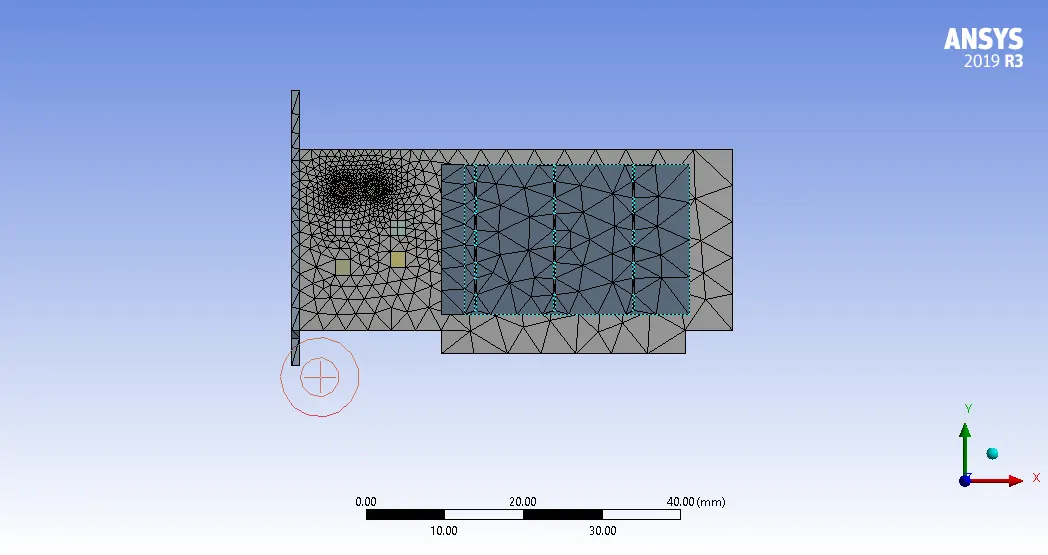
The meshing for the problem has been done for two cases,one is having a base line mesh and other is having a more refined meshing.

• Element Size : 10 mm
• Type of Mesh Elements : Tetrahedral
• Number of Elements : 84,805
• 

• 3.SETUP:

  Solver - Type : Pressure-Based

  - Velocity Formulation : Absolute

  - Time : Steady State

  Model - k-omega SST

  Material - Fluid : Air

  - Solid : Copper

  Aluminium

  Cell Zone Conditions - Processor

  • Type: Solid
  • Material : Cu

  • NOTE: The case has been simulated for various inet velocities from 1 m/s to 10 m/s and rest of all conditions remains unchanged

    Boundary Conditions - Inlet :

    • Velocity-inlet: CASE 1. 1 m/s

    CASE 2. 2 m/s

    CASE 3. 5 m/s

  • Thermal - Temperature 300 K

  - Oulet:

  • Pressure-outlet ( zero guage pressure )

  - Bottom-wall

  • No slip condition

  - Symmetry

  • Symmetry boundary condition

  • .4SOLUTION & RESULTS:

    • CASE 1. INLET VELOCITY 1 m/s

    1.Residual Plot:

    • 2.Temperature Contour Plot:

      3.Velocity Contour Plot:

    • CASE 2. INLET VELOCITY 2 m/s

    1. Residual Plot:

    • The solution converged at 55 iterations.

    2.Temperature Contour Plot:

    3.Velocity Contour Plot:

    • CASE 3. 5m/s

    1.Residual Plot:

    • The solution converged at 59 iterations.

    2.Temperature Contour Plot:

    3.Velocity Contour Plot:

    CONCLUSIONS:

    • The velocity at which the maximum heat transfer coefficient is obtained is 10 m/s
    • The potential hotspot in the system is that of the Processor.
    • The more refined the meshing especially along the components where the heat generation term is involved,the better the results will be as the problem will be more close towards the practical approach.
    • As the velocity is increased ,the Reynolds number will be increased which inturn increase the Nusselt number and heat transfer coefficient and further leading to better heat transfer rate
    • For the efficient cooling of the graphics card using the forced convection heat transfer, the velocity must be kept maximum within the practical limitations.