Week 7 Challenge

The challenge is to create a Vehicle model by taking Tractive force as input and also by considering the forces acting on the vehicle & vehicle dynamics and velocity as output. Here vehicle model here is nothing but the equations of forces which comes under vehicle dynamics i.e when vehicle moves from its rest position.

Forces acting on the Vehicle:

Vehicle needs a resultant force to come from rest position to motion and this resultant force is also known as Traction force. This traction force is provided by power train of a vehicle. But some resistive forces opposing this when vehicle starts moving.

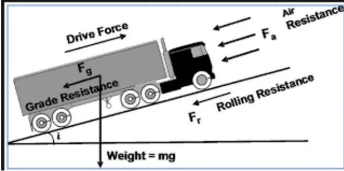
These resistance forces are

• Rolling resistance force(Frr).
• Aero dynamic force(Faero).
• Hill climbing force(Fhc).

To overcome these resistance forces additional traction force should be provided. The resultant traction force is

Resultant traction force = Traction force - (Fr + Faero + Fhc).

Simulink Model of Vehicle:

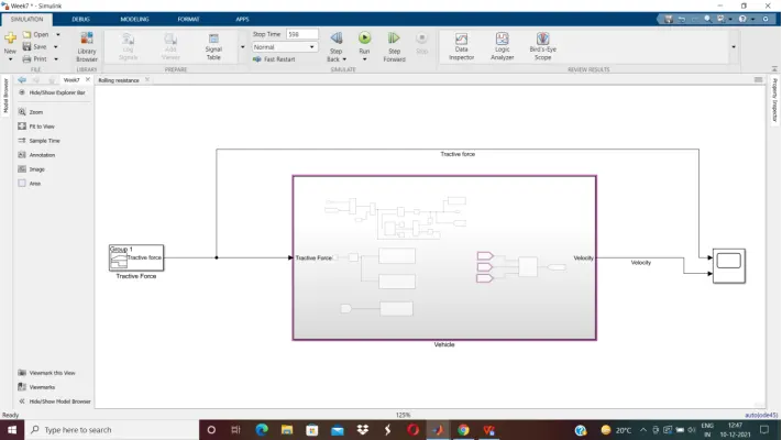
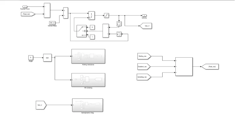
This is model with all the vehicle forces and dynamics with traction force as input and velocity as output. Inside subsystem we can observe all the blocks connected according vehicle equations.

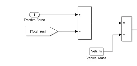
The top part model is to calculate resultant tractive force according to the equation by subtracting resistance forces from the tractive force. Then this is force is divided by mass to convert it into acceleration which is further integrated to get the velocity.

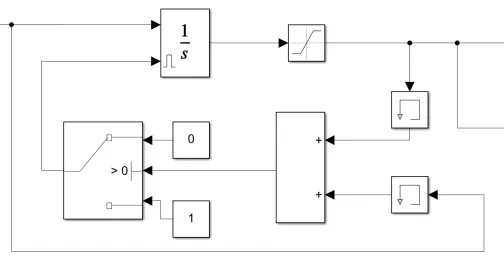
Here at Integrator, due to the integral windup the overshoot occurs. This windup can be overcome by using anti windup. This is obtained by using external reset by using switch and set reset values.

When the acceleration and velocity is not equal to zero, then external reset is set. When the acceleration and velocity is zero, then the external reset is reset.

By considering the initial condition of vehicle which is zero, in order to reject the unwanted errors, the memory is used.

Then the saturation block is used to get the forward velocity from zero to infinity.

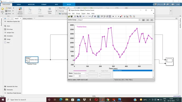
The tractive force is given as signal builder into which tractive force data is imported as shown below.

Resistance forces subsystems:

Rolling Resistance force:

Rolling resistance force is the force due to the friction of tyre and surface. Factors that contribute to rolling resistance are deformation of the wheels, the deformation of the roadbed surface, and movement below the surface Rolling resistance force can be formulated by multiplying the weight of the vehicle and coefficient of rolling resistance.

Frr=Veh_mass* g * Rolling resitance coeff * cos(alpha)

Veh_mass= 1200 kg

Roll reistance coeff = 0.015

G = 9.81 m/s

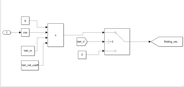
Here from the subsystem we can abserve that it is built according to the equation mentioned above. Here the switch block is used for considering the rolling resistance only when velocity is greater than 0 such that when vehicle is moving.

And it output Roll_Res taken as goto block which connects at the additions of all the reistance forces.

Aerodynamic Drag force:

Air Drag force is the force due to wind velocity opposing the vehicle on the frontal area. Air drag force on the vehicle is minimum when the vehicle is moving slowly. If the speed increases, the air drag force also increases. This creates the opposing force on the vehicle. Air drag force can be identified by using the formula.

Faero = (1/2)*Cd*Af* delta*Veh_V^2

Cd = Drag coefficient = 0.2

Af = Frontal area = 1.97 m^2

Delta = Air density = 1.225 kg/m^3

V = Velocity of vehicle in m/s

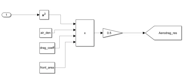
This is the Aerodynamic drag force subsystem which is according to the Faero equation.

Hill Climbing force:

Hill climbing force (grade resistance) is the force acting against the direction of acceleration of vehicle when the vehicle moving at a certain angle (slope). This force is acting in opposite due to gravity.

Fhc=Veh_mass * g * sin (alpha)

Veh_mass = Mass of the vehicle =1200 kg

g = gravity = 9.81 m/s

alpha = angle in radians

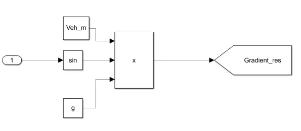
This is the Hill climbing force subsystem which is according to the Fhc equation.

All these forces are added to get the Total resistance forces as shown below.

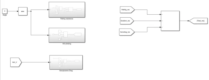
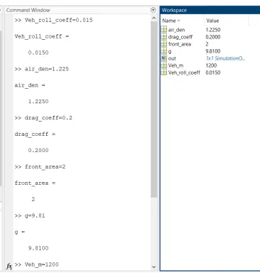
The parameters are initialised in the command window, thus saved to the workspace as shown.

Result:

Here the scope is connected to the input tractive force and the output Velocity and simulation is run for 598 sec.

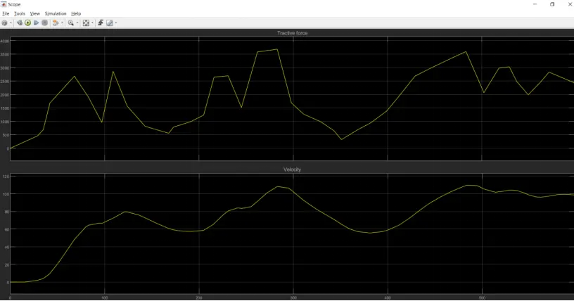
From the plot we can observe the tractive force and velocity graphs. And by comparing them we can observe that whenever the tractive force is increasing then the velocity of the vehicle is increasing and when traction force is decreasing then velocity is decreasing.

And we can also observe that for first few seconds the velocity is still even when the traction force is increasing and this is due to resistance forces that opposing the vehicle velocity.

Thus vehicle model is created considering the force acting on the vehicle & vehicle dynamics.