Week 7 Challenge

AIM/OBJECTIVE:

• Vehicle modelling
• Vehicle dynamics
• Force and output velocity

VEHICLE MODEL IN MATLAB SIMULINK:

Vehicle model here is nothing but the equations of forces which comes under vehicle dynamics i.e when vehicle moves from its rest position. For motorized vehicles, such as automobiles, aircraft, and watercraft, vehicle dynamics is the study of vehicle motion, e.g., how a vehicle's forward movement changes in response to driver inputs, propulsion system outputs, ambient conditions, air/surface/water conditions, etc. Below image shows the force acting on a vehicle.

Where

• Ftr-tractive force;
• Fa-aerodynamic drag resistance force;
• Fg-gradient resistance force;
• Fr-rolling resistance force;
• Fi-inertial resistance force 

Tractive force is the force applied/produced by the vehicle powertrain. We will now see the equations of three main forces (aero, rolling and gradient) and will implement this using matlab Fcn block.

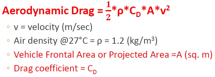
Aero dynamic drag: Aerodynamic Drag is a force which the oncoming air applies on a moving body. It is the resistance offered by the air to the movement of the body. So, when a car is moving; it displaces the air. However, it affects the car’s speed and performance. Technically, it is the aerodynamic drag or the friction offered by the air to a vehicle.

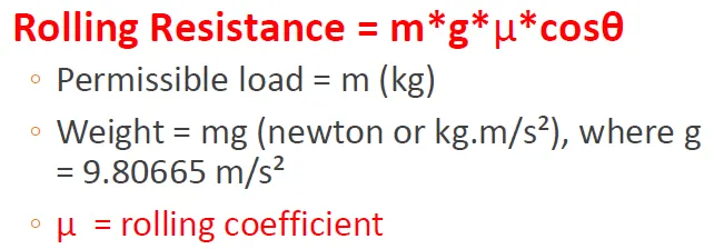
Rolling resistance force: Rolling resistance is the combination of forces that work against the forward motion of your vehicle. The weight of the vehicle, gravity and inertia, the amount of friction between the tires and the road surface, and air drag all play a part. When you coast in your car or on a bike, rolling resistance is what slows you down. The more rolling resistance, the more power it takes to propel a vehicle.

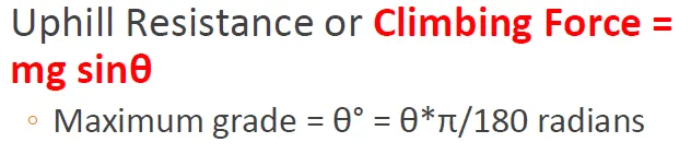
Gradient/uphill/climbing force: When the vehicle travels uphill, a component of its weight works in a direction opposite to its motion. If some energy is not supplied to overcome this backward force, then the vehicle would slow down, stall and roll backwards.

Force of acceleration: The acceleration force refers to the vehicle’s resistance to speed variations. This force holds you back when you increase your speed and also moves you forward when you slow down. In other words, it means that you consume energy to accelerate up to a certain speed but can recover part of that energy when you decelerate, allowing you to drive a certain distance without consuming fuel. In equations it is simply written as:

F=m*a (where m is the mass of object(vehicle) and a is acceleration)

VEHICLE MODEL:

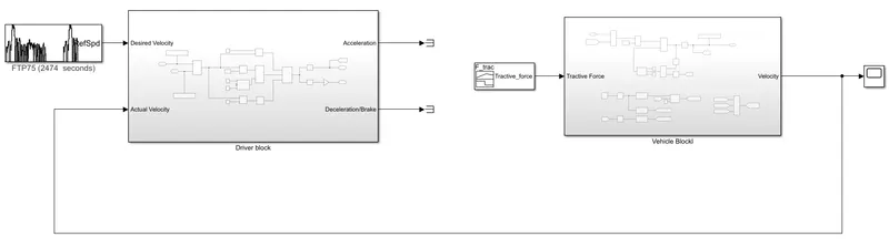
The model shown above shows driver block too but our focus is on vehicle block only. Driver block is used here because we need acceleration value to overcome the integral wind up happening while converting tractive force into velocity. Hence only vehicle blocks system and its explaination is done here.

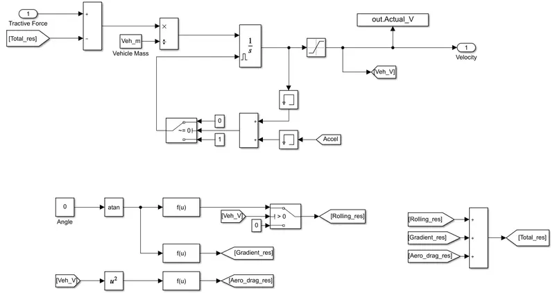
Inside view of vehicle block is shown below:

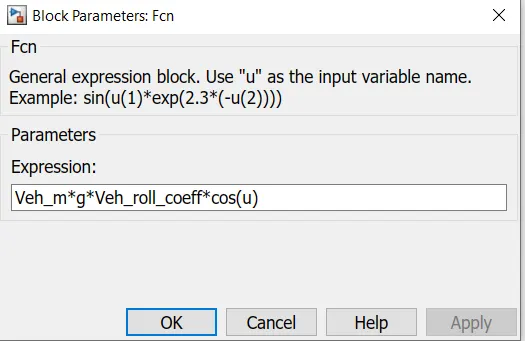
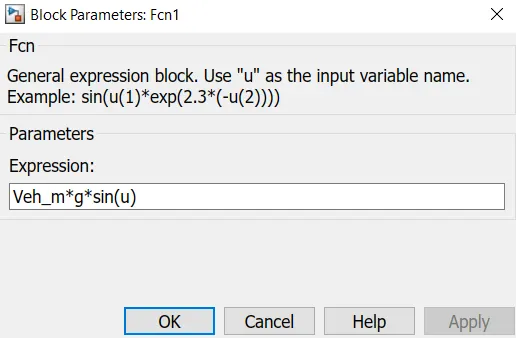
Drag force, gradient force and rolling resistance force implemented using Fcb block:

  

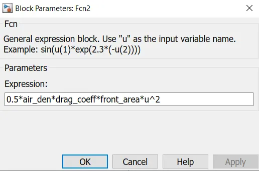
We will understand Rest all thing about model while explaining its working.

WORKING OF MODEL

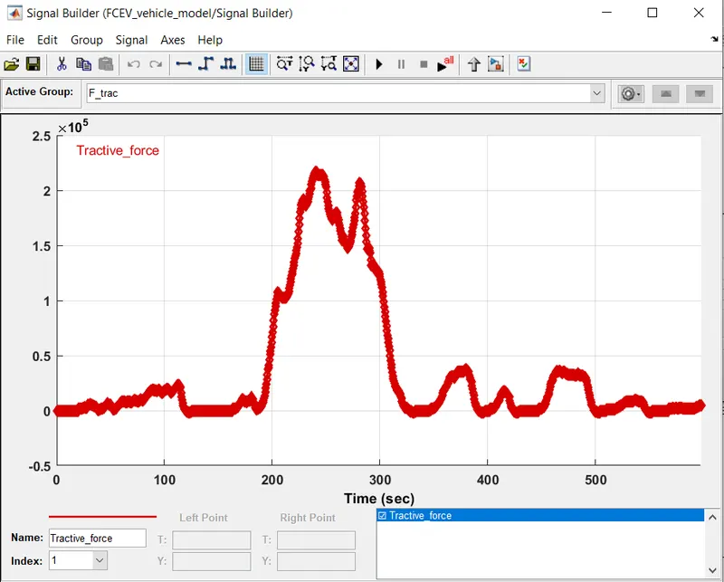
1. The input to the vehicle block is tractive force. This tractive force is the force which is applied by the powertrain to the vehicle body. We have given tractive force directly as a input. Its values are in newton. Its plot (of values) is shown below:

2. Now comes directly the main part, i.e to find velocity. We know the sum of all the forces acting on vehicle is force of traction which is given as:

F_trac = Force of acclereation(Fa) + Rolling resistance force(Fr) + Gradient force(Fg) + aerodynamic force(Fd) 

The term force of of acclereation (Fa=m*a) will help us to find the velocity (Mathematically). We will first seperate the accleration term and resistive force terms.

F_trac-Fr-Fg-Fd = Fa

F_trac-Fr-Fg-Fd = m*a

`(Ftrac-Fr-Fg-Fd)/m = a`

so we now have acclerartion with us. (Follow mathematically)

3. The forces other than F_trac in model is calculated (of which formula implemention using Fcn block is already shown) as shown below: 

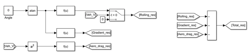
• We have taken grade as Zero hence there will be no gradient force acting on vehicle.
• Fr is independent of velocity value but only acts on vehicle when its moving. Hence switch is used to make sure the force is taken into account only when velocity is of some value.
• Aerodynamic force or drag force is purely a function of square of velocity. Hence the Fcn block is given velocity square as its function. 
• Sum of these forces is then substracted with tractive force.

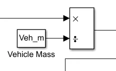
4. Then after this the result of above procedure is divided by mass to get the acceleration value:

5. Now we have acceleration with us. We know that acceleration is the rate of change of velocity i.e the derivative of velocity. Hence its anti-derivation or integration will give us the velocity. What been said theoritically is actually implemented in Simulink using required blocks:

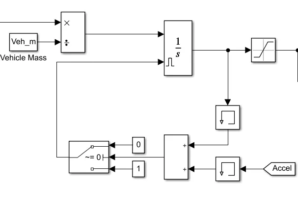
We have also taken here of integral wind up. Integral windup particularly occurs as a limitation of physical systems, compared with ideal systems, due to the ideal output being physically impossible (process saturation: the output of the process being limited at the top or bottom of its scale, making the error constant). For example, the position of a valve cannot be any more open than fully open and also cannot be closed any more than fully closed. In this case, anti-windup can actually involve the integrator being turned off for periods of time until the response falls back into an acceptable range. As soon as the acc. and velocity goes zero the reset button gets active.

6. Saturation block makes it sure that our velocity is within the defined limits. Here we the upper value is infinity because we werent sure of the tractive force effect on vehicle.

7. The vehicle parameters is loaded using .mat files. The parameters value is shown below:

Parameter	Value
Vehicle mass	1200 Kg
Gravitational force	9.81
RR coefficient	0.013
Air density	1.2
Drag coeff.	2.5
Grade or Angle	0

Simulation Results:

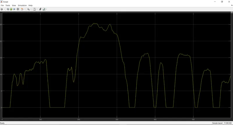
Output velocity: