Project
CHALLENGE/AIM: Carry out a system-level simulation of an all-terrain vehicle.
OBJECTIVE: Prepare a technical report explaining the model properties & comments on the results
HISTORY OF/ABOUT BAJA ATV (All terrain vehicle):
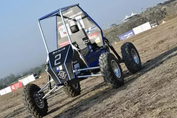
ATV or All Terrain Vehicles are a vehicle that travels on low-pressure tires, with a seat that is straddled by the operator, along with handlebars for steering control. As the name implies, it is designed to handle a wider variety of terrain than most other vehicles
Now Baja California is a sovereign state in Mexico peninsula.
A lot of Dune bashing/Racing used to take place in the sand dunes of Baja California and these races came to be known as Baja Races. Now to adopt with these dunes specific modifications were made to cars iconic amongst which was the Baja Bug which was nothing but a VW Beetle modified for the Baja Dunes.
In 1976 the University of Southern California held the first ATV event which was named Baja SAE keeping in mind the popularity of the races in the Baja Dunes at that time. As time progressed the event became quite famous and the ATVs that were made for the purpose of the competition began to be referred to as Bajas.
An ATV that abides by certain rulesets that are devised by the SAE for a competition is known as Bajas.
ABOUT BAJA ATV SIMULINK MODEL:
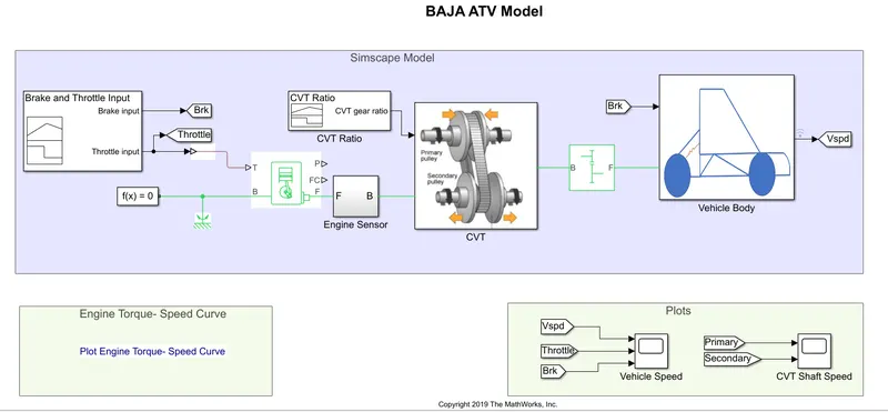
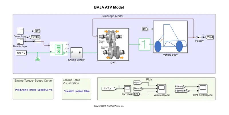
Now this model named BAJA ATV was made to give a kick start to the people who wanted to design the baja atv using MATLAB simulink software. To get better understanding of this model we will explain it by component wise and by then observing the various results we will make our comment.
Further this model is divided into 4 categories:
1. BAJA ATV model (open loop)
2. BAJA ATV model with DASHBOARD (Changing or giving input while simulation is running) (open loop)
3. BAJA ATV model with closed loop system (Giving mapped values of CVT ratio Vs. vehicle velocity as input )
4. BAJA ATV model with closed loop system and DASHBOARD.
But we will first explain some components in model using basic BAJA ATV model which is first of the categories:
EXPLAINATION OF SOME COMPONENTS IN MODEL:
Generic Engine block
The Generic Engine block represents a general internal combustion engine. Engine types include spark-ignition and diesel. Speed-power and speed-torque parameterizations are provided. A throttle physical signal input specifies the normalized engine torque. Optional dynamic parameters include crankshaft inertia and response time lag. A physical signal port outputs engine fuel consumption rate based on choice of fuel consumption model. Optional speed and redline controllers prevent engine stall and enable cruise control.
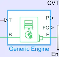
By default, the Generic Engine model uses a programmed relationship between torque and speed, modulated by the throttle signal.
Engine Speed, Throttle, Power, and Torque
The engine model is specified by an engine power demand function g(Ω). The function provides the maximum power available for a given engine speed Ω. The block parameters (maximum power, speed at maximum power, and maximum speed) normalize this function to physical maximum torque and speed values.
The normalized throttle input signal T specifies the actual engine power. The power is delivered as a fraction of the maximum power possible in a steady state at a fixed engine speed. It modulates the actual power delivered, P, from the engine: P(Ω,T) = T·g(Ω). The engine torque is τ = P/Ω.
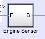
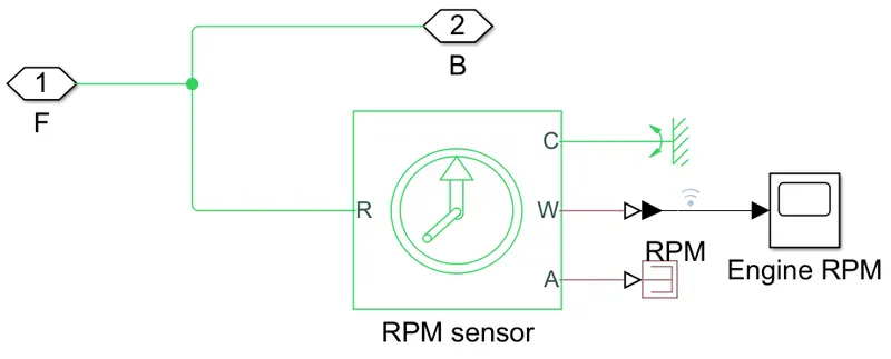
Engine sensor
Inside this block there is ideal rotational motion sensor which is used to plot the engine rpm.
CVT (continuously variable transmission)
ABOUT CVT:
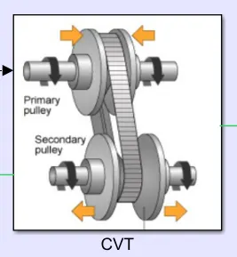
A continuously variable transmission (CVT) is an automatic transmission that can change seamlessly through a continuous range of gear ratios. This contrasts with other transmissions that provide a limited number of gear ratios in fixed steps. The flexibility of a CVT with suitable control may allow the engine to operate at a constant RPM while the vehicle moves at varying speeds.
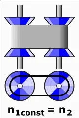
CVTs are used in automobiles, tractors, motor scooters, snowmobiles, and earthmoving equipment.
The most common type of CVT uses two pulleys connected by a belt or chain, however, several other designs have also been used at times.
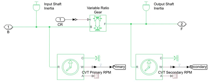
CVT Model:
VARIABLE RATIO GEAR:
The Variable Ratio Transmission block represents a gearbox that dynamically transfers motion and torque between the two connected driveshaft axes, base and follower.
Ignoring the dynamics of transmission compliance, the driveshafts are constrained to corotate with a variable gear ratio that you control. You can choose whether the follower axis rotates in the same or opposite direction as the base axis. If they rotate in the same direction, ωF and ωB have the same sign. If they rotate in opposite directions, ωF and ωB have opposite signs.
Transmission compliance introduces internal time delay between the axis motions. Therefore, unlike a gear, a variable ratio transmission does not act as a kinematic constraint. You can also control torque loss caused by transmission and viscous losses. For model details, see Variable Ratio Transmission Model.
Ports
B and F are rotational conserving ports representing, respectively, the base and follower driveshafts.
You specify the unitless variable gear ratio gFB(t) as a function of time at the physical signal input at port r. If the signal value becomes zero or negative, the simulation stops with an error.
INPUT/OUTPUT SHAFT INERTIA:
The Inertia block represents an ideal mechanical translational inertia, described with the following equation:
T=Jdωdt
where:
-
T is inertia torque.
-
J is inertia.
-
ω is angular velocity.
-
t is time.
By default, the block has one mechanical translational conserving port. The block positive direction is from its port to the reference point. This means that the inertia torque is positive if inertia is accelerated in positive direction.
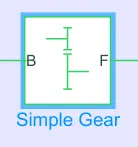
SIMPLE GEAR:
Purpose of using this block is for speed reduction. It is just a simple mechanical system.
VEHICLE BODY:
VEHICLE BODY:
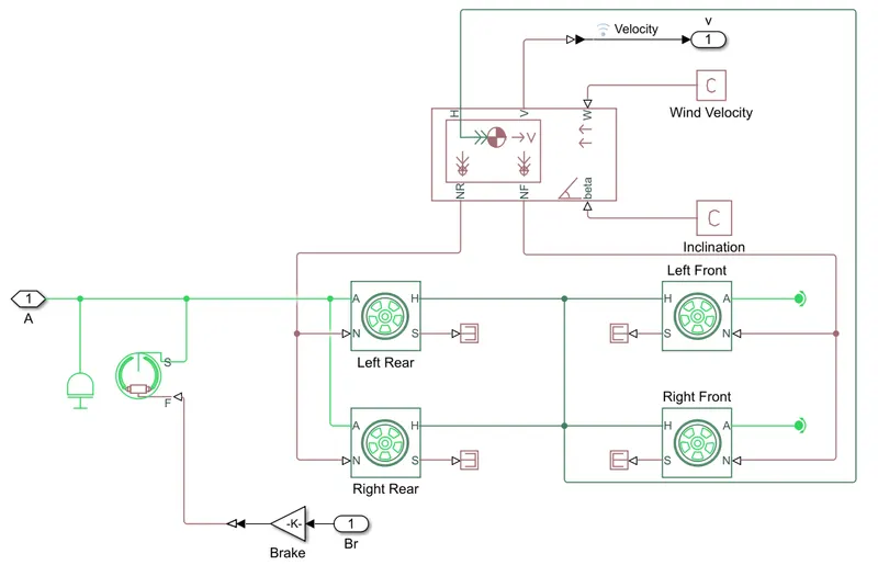
The Vehicle Body block represents a two-axle vehicle body in longitudinal motion. The vehicle can have the same or a different number of wheels on each axle. For example, two wheels on the front axle and one wheel on the rear axle. The vehicle wheels are assumed identical in size. The vehicle can also have a center of gravity (CG) that is at or below the plane of travel.
The block accounts for body mass, aerodynamic drag, road incline, and weight distribution between axles due to acceleration and road profile. Optionally include pitch and suspension dynamics. The vehicle does not move vertically relative to the ground.
The block has an option to include an externally-defined mass and an externally-defined inertia. The mass, inertia, and center of gravity of the vehicle body can vary over the course of simulation in response to system changes.
MODEL
The vehicle axles are parallel and form a plane. The longitudinal, x, direction lies in this plane and perpendicular to the axles. If the vehicle is traveling on an incline slope, β, the normal, z, direction is not parallel to gravity but is always perpendicular to the axle-longitudinal plane.
TIRE( MAGIC FORMULA):
The Tire (Magic Formula) block models a tire with longitudinal behavior given by the Magic Formula [1], an empirical equation based on four fitting coefficients. The block can model tire dynamics under constant or variable pavement conditions.
The longitudinal direction of the tire is the same as its direction of motion as it rolls on pavement. This block is a structural component based on the Tire-Road Interaction (Magic Formula) block.
To increase the fidelity of the tire model, you can specify properties such as tire compliance, inertia, and rolling resistance. However, these properties increase the complexity of the tire model and can slow down simulation. Consider ignoring tire compliance and inertia if simulating the model in real time or if preparing the model for hardware-in-the-loop (HIL) simulation.
TIRE MODEL
The Tire (Magic Formula) block models the tire as a rigid wheel-tire combination in contact with the road and subject to slip. When torque is applied to the wheel axle, the tire pushes on the ground (while subject to contact friction) and transfers the resulting reaction as a force back on the wheel. This action pushes the wheel forward or backward. If you include the optional tire compliance, the tire also flexibly deforms under load.
DOUBLE-SHOE BRAKE BLOCK:
The Double-Shoe Brake block represents a frictional brake with two pivoted rigid shoes that press against a rotating drum to produce a braking action. The rigid shoes sit inside or outside the rotating drum in a diametrically opposed configuration. A positive actuating force causes the rigid shoes to press against the rotating drum. Viscous and contact friction between the drum and the rigid shoe surfaces cause the rotating drum to decelerate.
Double-shoe brakes provide high braking torque with small actuator deflections in applications that include motor vehicles and some heavy machinery. The model employs a simple parameterization with readily accessible brake geometry and friction parameters.
You can also enable faulting. When faulting occurs, the belt will exert a user-specified force. Faults can occur at a specified time or due to an external trigger at port T.
SIMULATION RESULTS WITH EXPLAINATIONS:
1.BAJA ATV model without dashboard (openloop):
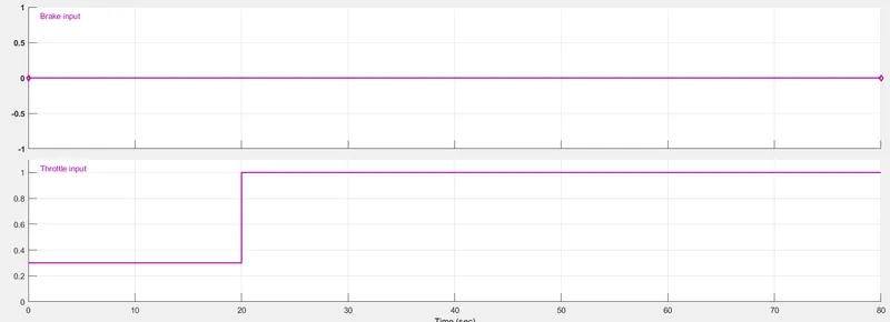
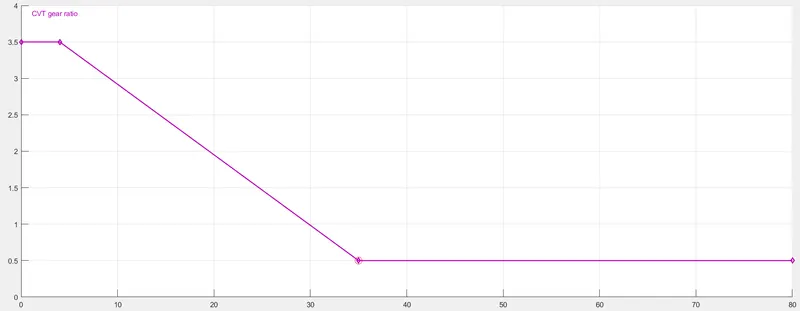
In this model we are using Signal builder to give a input. Inputs from our side are brake and throttle and CVT ratio. Brake input is zero throughout the simulation and throttle is 0.3 for 0 to 20 secs and 1 beyond it. CVT ratio is 3.5 for 0 to 4 secs then it linearly decreases to 0.5 in time span of 4 to 35 secs and after this it stays constant.
INPUTS
OUTPUT
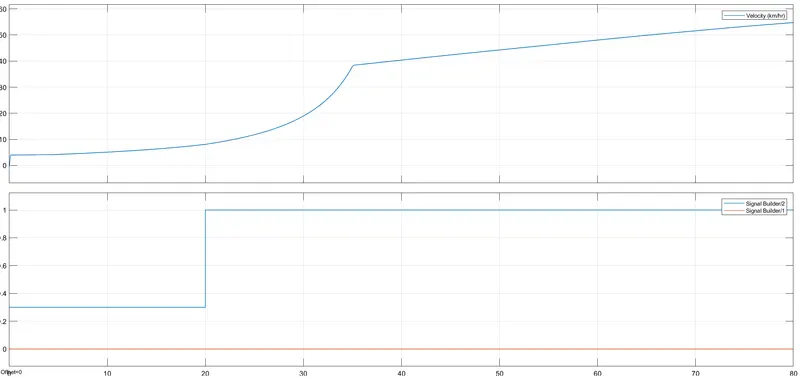
From above fig. we can see that with increase in throttle input speed also gets increased and finally attains max speed.
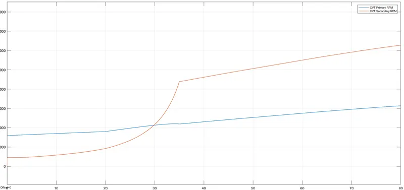
The fig below plots CVT shaft speed which is primary and secondary CVT shaft. What you will observe here is that secondary rpm is increasing with decrease in CVT ratio. Because speed here is directly proprtional to radius. With this we can also observe that CVT has adjusted speed various number of gear ratios.
BAJA ATV model with dashboard:
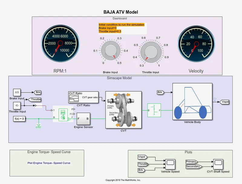
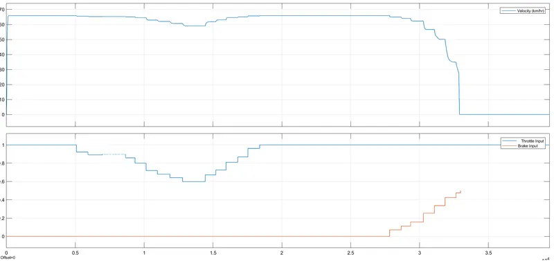
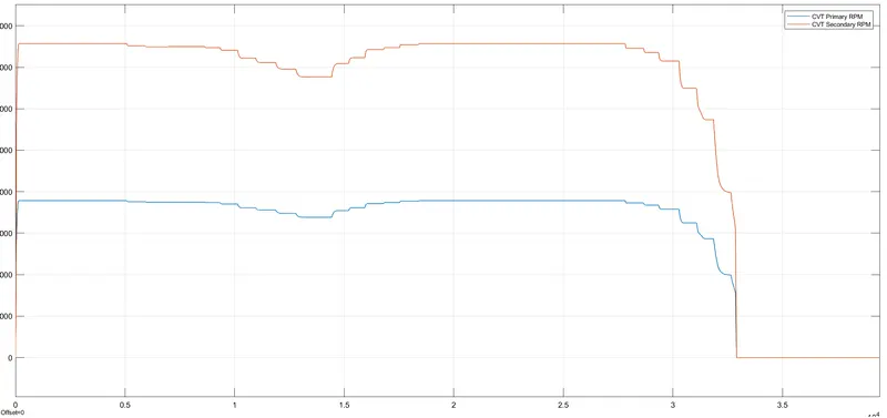
Now there is not much diffrence between the model with and without dashboard except we are giving input while simulation is running. Intially the brake input is zero and throttle input is 1. Intentionally we have just decrease and increased the throttle speed and brake input is increased to 0.5. Results are shown below and it is evident that our models output did vary as input given.
BAJA ATV model (Closed loop) using mapped values of CVT ratio
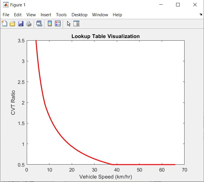
As we all know giving random values as CVT ratio is not realisitic because CVT ratio always depend on velocity thats why there is one more that is closed loop model using lookup table. For that we have used data of previous cvt model and the code is given below:

Results
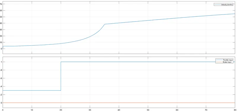
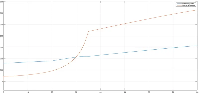
It can be seen in the result plot that our model worked just as the mapped values of CVT gear ratio were given. these mapped values are taken by running our first openloop model.
BAJA ATV model (Closed loop) with dashboard:
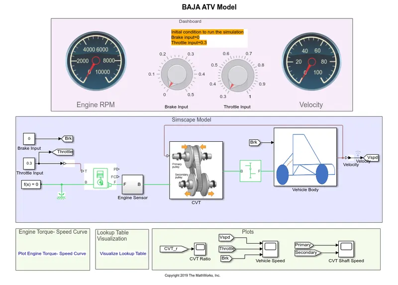
Now to give input or change the input whilw the simulation is running we have built this model which is our main purpose. Rest model is exactly similar to that which has no dashboard.
Results
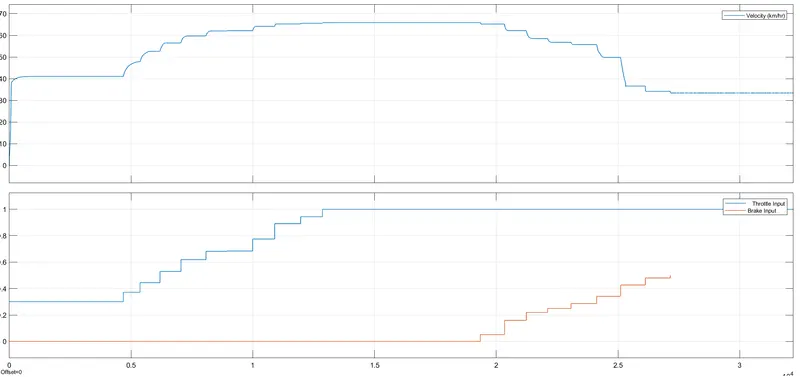
CVT (Primary Vs secondary rpm)
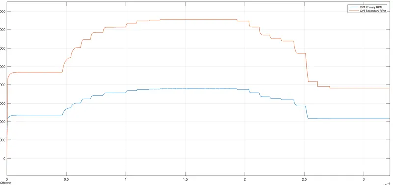
Hence it can be concluded from the results that our model did run as we designed it for.
CONCLUSION: Baja ATV is unique in its kind. By making a simulink model of it we have succesfully visualise how CVT can incerase the effeciency of ATV. We have also done various simulation with defined inputs and run time inputs which made our conclusion stronger. With this model one can start to build its own BAJA type ATV.