Week 7 Challenge

• The vehicle when moving on the road has various forces acting on it.
• When longitudinal forces and lateral forces are considered in the model, it becomes a 2D model.
• The lateral forces are not considered for this model thus making it a 2D model.

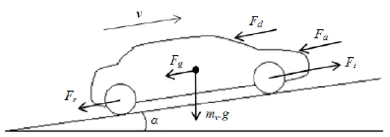
where

Ft = Tractive Force
Fa = Aerodynamic Drag Force
Fg = Gradient Resistance Force
Fr = Rolling Resistance Force
Mv = Mass of the vehicle
g = Gravitational acceleration (= 9.81 m/s^2)
v = Velocity of the vehicle

• The electric powertrain block does all the signal processing and generates a tractive/propulsion force.
• This is then fed into the vehicle model block.
• The tractive force propels the vehicle model block.
• The tractive force propels the vehicle forward overcoming the resistance it faces.

i. Rolling Resistance Force:

• Rolling resistance is friction or the force resisting the motion of a circular object that's rolling on a surface.
• For modern radial tires, there is a deflection in the part of the tire which is in contact with the road surface.
• This causes the normal force to shift.
• The normal force is higher in the frontal part of the tire in contact with the ground due to this shift.
• This shift in the normal force causes a moment about the centre of rotation which acts in the opposite direction.

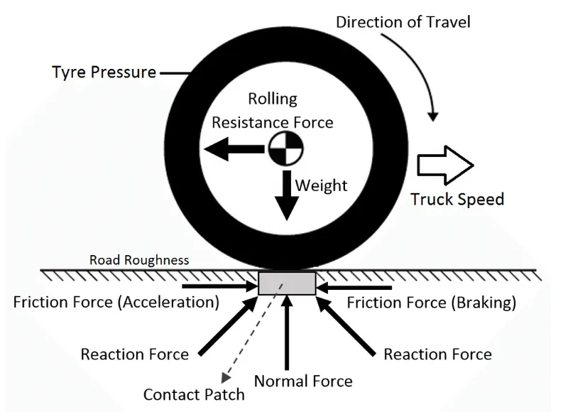
• The distance of shift in the normal force is a and Fz denotes the normal force.
• To overcome this resistance, the force needed to be applied to the centre of the wheel comes out to be
  
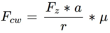
• In the equation, r is the effective rolling radius of the tire and μ is the rolling resistance coefficient. The above force is only when the vehicle is on a straight road.
• When going on a slope, a cosine component of the force is needed to propel the vehicle forward.
• For a vehicle on a road with a slope α, it turns out to be
  
• For a vehicle running on dry asphalt, an approximate assumption for the value of coefficient friction was made to be 0.015.
• P is the normal force and the acceleration causing that force is gravity at 9.8 m/s^2.
• So, the equation above can be rewritten with Mv being the mass of the vehicle as
  

ii. Aerodynamic Drag:

• This resistance is directly proportional to the speed of the vehicle.
• Along with the velocity of the vehicle, the amount of aerodynamic drag a vehicle faces also depends on the front shape of the vehicle or the frontal area.
• The vehicle when moving forward leaves behind an area of low air pressure.
• As per the rule of physics, air flows from a high-pressure area to a low-pressure area thus increasing the aerodynamic resistance.
• Considering all the factors, the equation for the aerodynamic drag can be defined as:
  
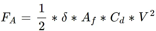
  δ = Density of the surrounding air
  Cd = Drag Coefficient
  Af = Vehicle frontal area
  V = Velocity of the vehicle

iii. Grade Resistance:

• When a car is going uphill, it experiences an additional resistance component which is due to the grade of the road and it's called grade resistance.
• But when going downhill, it helps in the motion of the vehicle.
• The amount of grade resistance or assistance depends on the mass of the vehicle denoted as M and is defined as
  

Simulink Model:

i. Driver Subsystem:

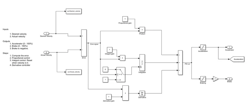
• In this subsystem, two inputs are created: Desired Velocity & Actual Velocity and two outputs are created: Accelerator & Brake.
• According to the session, we followed the steps:
  i. Compute the error: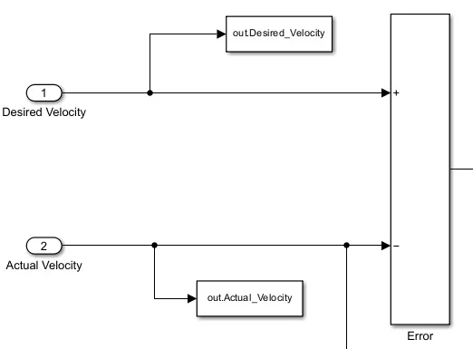
  
  In the first step, we'll connect the Desired velocity (Drive Cycle Source) and the Actual velocity (output) to the subtract block. This helps us in calculating the error occurring between them.
  
  ii. Proportional control: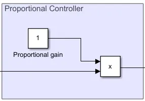
  
  The proportional component depends only on the difference between the desired velocity and the actual velocity. In this step, we'll design the Proportional Controller by using a constant as the proportional gain and error signal. These two inputs are connected to a Product block which gives us the proportional response.
  
  iii. Integral Control reset when velocity is 0: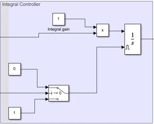
  
  The integral component sums the error over time. The result is that even a small error term will cause the integral component to increase slowly. The integral response will continually increase over time unless the error is zero, so the effect is to drive the Steady-State error to zero. Steady-State error is the final difference between the actual velocity and desired velocity. A phenomenon called integral windup results when integral action saturates a controller without the controller driving the error signal toward zero. In this step, the product of the Integral gain and error signal will be integrated with respect to time by using the Integrator Block.
  
  iv. Derivative Controller: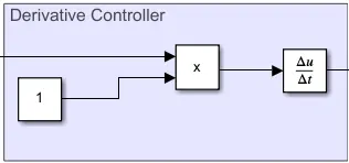
  
  The derivative component causes the output to decrease if the process variable is increasing rapidly. The derivative response is proportional to the rate of change of the process variable. Increasing the derivative time parameter will cause the control system to react more strongly to changes in the error term and will increase the speed of the overall control system response.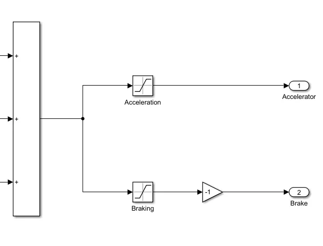
  
  
  From this PID Controller output, we have to create the acceleration and brake commands by using the Saturation blocks.
  
  Acceleration saturation block consists of the following parameter values.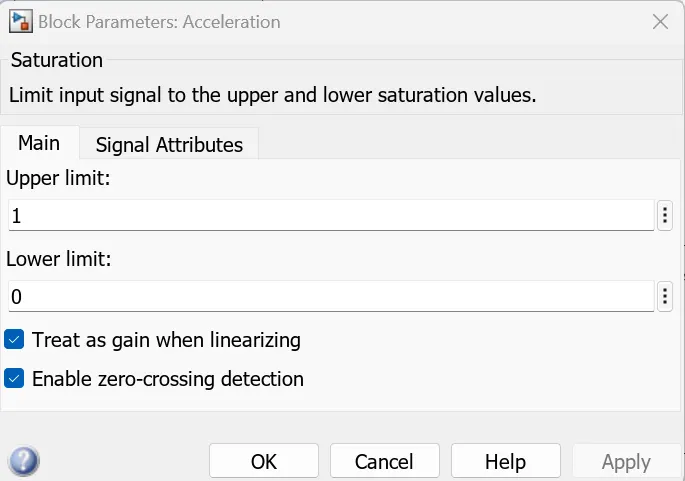
  
  
  The brake saturation block consists following parameter values.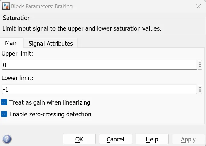
  
  Since there is no negative velocity in this model, we are using the negative gain block for getting the Positive velocity as Output.

ii. Vehicle Subsystem:

• We know that
  Force = Mass * Acceleration
  then,
  Acceleration = Force/Mass
  
  
  
• But here the force is subtracted from the actual force to the total traction force.
  
  The total traction force is
  Ft = Frr + Fa + Fg
  where,
  Ft = Total force
  Frr = Rolling resistance force
  Fa = Aerodynamic Drag force
  Fg = Grade force

Rolling Resistance Force

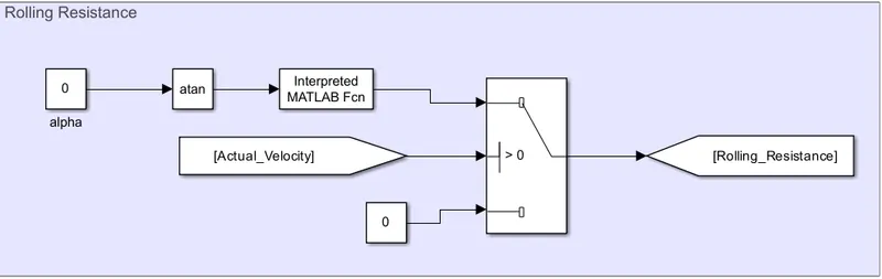
The force is implemented by using the Interpreted MATLAB Fcn.

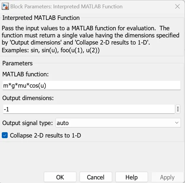
Aerodynamic Drag Force

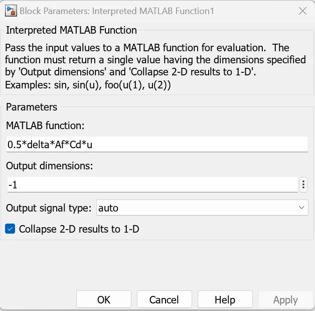
Grading Force

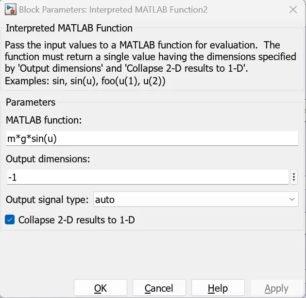
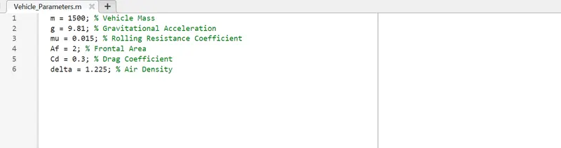
The values are defined in the MATLAB command window as follows:

Total Resistance Force

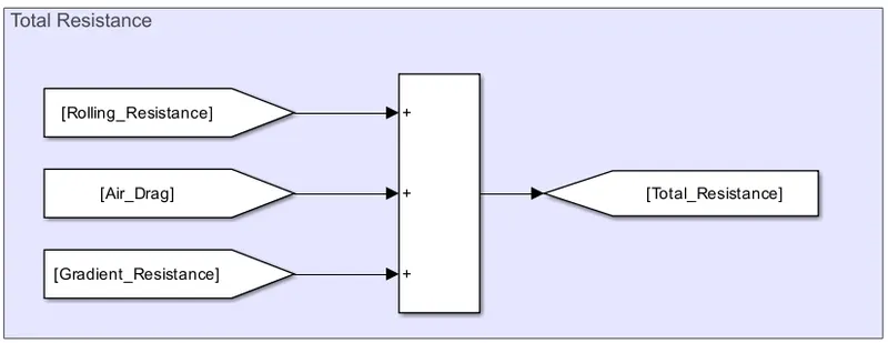
The above forces are added to provide the total resistance force.

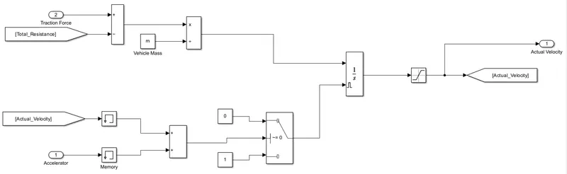
This total resistance force is subtracted from the given traction force whose difference is divided by the vehicle mass to provide acceleration. This acceleration is again integrated with respect to time to provide actual velocity.

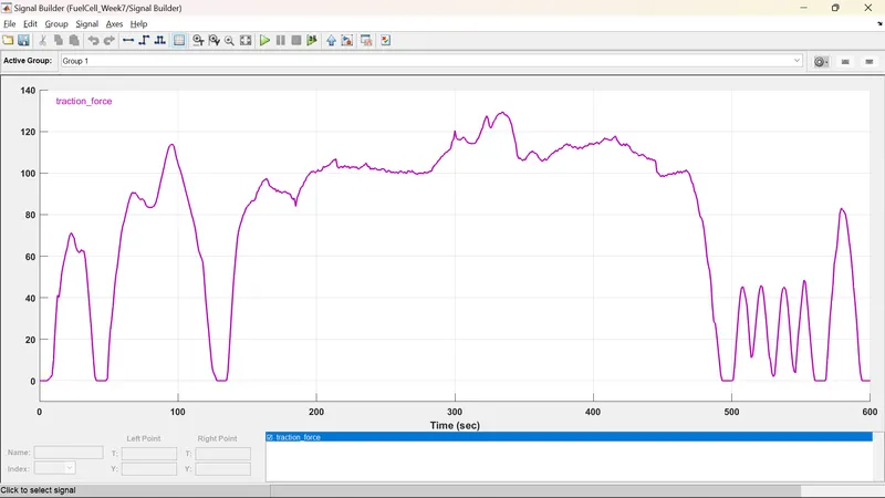
Output

After simulating for 598 sec, we get the graphical representation of the Drive Cycle and Vehicle Velocity.

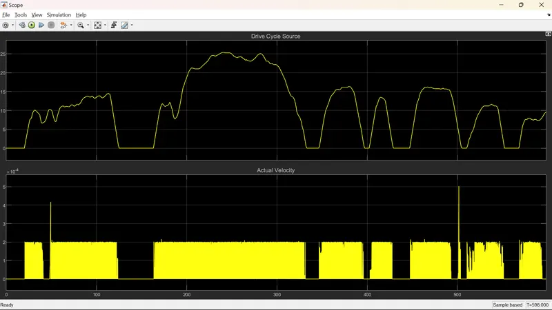
Here, we can see that the vehicle is operated by using the drive cycle source. The velocity has been plotted for the period of t = 598 sec.

Conclusion:

The vehicle parameters are loaded. The vehicle model is completed and the simulation stop time is set to 598 sec.