Week 7 Challenge
Load the vehicle parameters. Complete the vehicle model by modelling the remaining equations. Set simulation stop time to 598 sec.
The output should be the vehicle velocity.
Aim: Construct simulink model for vehicle body.
Objective:
- Load the vehicle parameters.
- We have to construct model using driver block,traction force, Vehicle dynamics.
- Simulation time set to 598 sec.
Introduction:
What is a vehicle body?
The vehicle body could be the main supporting structure or its particular element. The Vehicle Body of a modern car consists of an engine section, saloon, and trunk. The vehicle body is the main supporting structure of a vehicle, to which all other components are attached. The truck uses a separate frame as chassis.
Traction force:
The force used to produce or create motion by the use of dry friction between a body and a tangential surface is known as traction or tractive force. To create friction, commonly, the shear force of the surface is also used.
What is Traction or Tractive Force?
Traction is often expressed as the ratio or fraction of the maximum tractive force to the normal force
when the maximum tractive force between a body and a surface is limited by the available friction.
When this happens, it is generally called the coefficient of traction, which is similar to the coefficient
of friction. By overcoming all the resisting forces like air resistance, rolling resistance, friction,
normal loads, etc., this force makes an object move over a particular surface. Hence, traction is a
physical process that uses dry friction and transmits a tangential force across an interface between
two bodies.
Coefficient of traction:
The ratio or fraction of the force of friction between two bodies and the force pressing them together
is known as COF – coefficient of friction, often denoted by µ; it is a dimensionless scalar quantity.
The materials used are a major factor on which the coefficient of friction depends. For instance, steel
on ice has a small coefficient of friction as compared to rubber on pavement, which will have a
high coefficient of friction.
The range of coefficients of friction is nearly zero to greater than one. Between two surfaces of
different metals, the coefficient of friction will have a low value, and between two similar metals, the
coefficient of friction will have a greater value. For instance, copper has a higher coefficient of
friction when moved against copper but less if moved against brass or aluminum.
The force for traction, which is usually divided by the weight on the running gear such as wheels,
tracks etc., is known as the coefficient of traction.
Coefficient of traction = Usable traction / Normal force
What is Frictional force?
When the surface of one object comes in contact with the surface of another, then there exists a
force that resists motion between them, and that force is known as frictional force. A machine’s work
output is reduced by friction; in other words, we can say that because of friction, the ratio of output
to input is reduced.
Similarly, one-quarter of the energy of an automobile is used to counteract the limiting friction. Yet,
friction is important because it allows the tires of the car to stay on the road, and on the other hand,
friction present in the clutches makes it possible to drive. Friction is one of the most substantial
phenomena, from matches to machines to molecular structures, in the physical world.
Here are a few factors that affect the force of friction:
- The texture of the surface and the amount of force driving them together is the main cause that affects the frictional force.
- The amount of frictional force also gets affected by the angle and position of the object.
- The frictional force will be equivalent to the weight of an object if that object is placed flat against any other object.
- The frictional force will be improved if an object is pushed against the surface and becomes more than the weight of the object.
Rolling resistance sometimes called rolling friction or rolling drag, is the force resisting the motion when a body (such as a ball, tire, or wheel) rolls on a surface.
In this simulation Formulae used are:
- Rolling Resistance, Fr = M * g * µ * cos(α)
- Aerodynamic drag, Fad = 0.5 * Cd * Af * ρ * V^2
- Grade Resistance ,Fg = M*g*sin(α)
Simulink model:
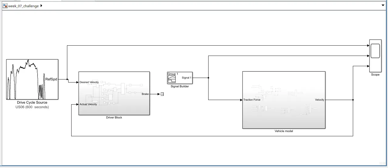
Above Simulink model consist of 3 Subsystems. They are,
- Driver block
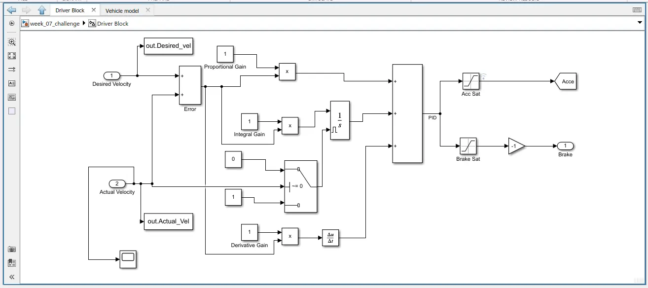
- Vehicle Model
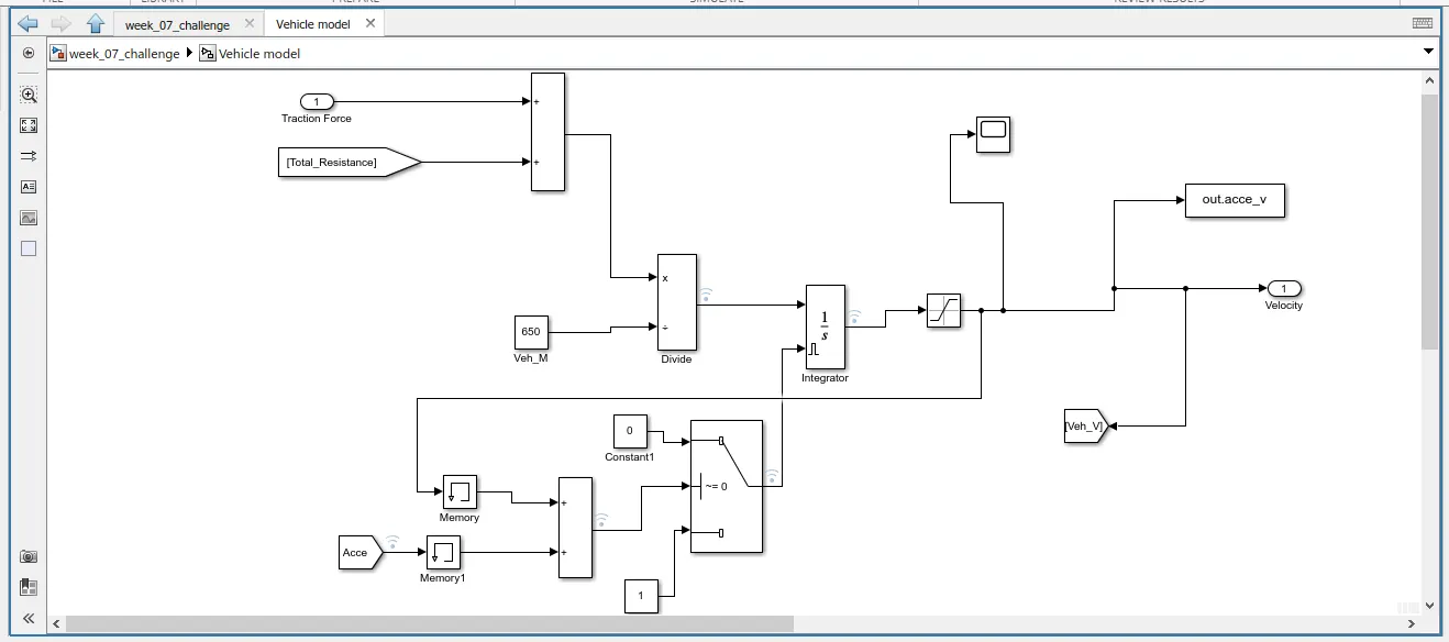
- Resistive force block
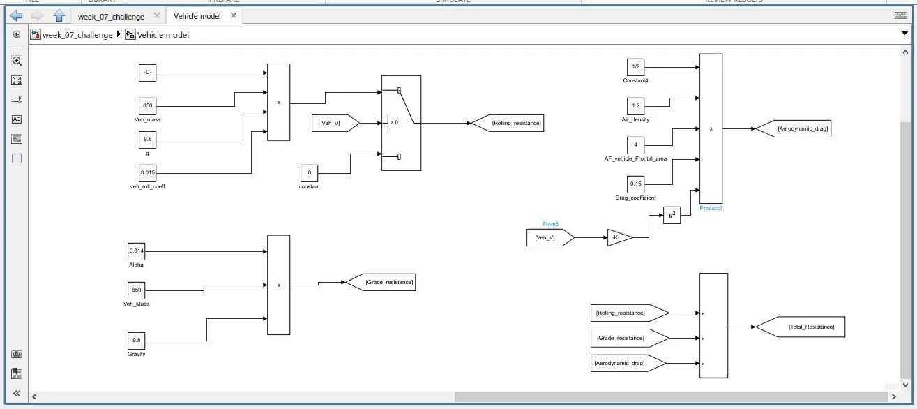
List of components used in this simulations:
- Constant block
- Goto block
- From block
- Product block
- Add block
- Scope block
- Signal builder block
- Drive cycle source
- Switch
- To workspace
- Gain block
- saturation block
- Derivative block
- Integrator block
- Import/outport block
- Memory block, etc.
Detail about some of the important blocks from the list given above;
- Memory block
The Memory block holds and delays its input by one major integration time step. When
placed in an iterator subsystem, it holds and delays its input by one iteration. This block accepts
continuous and discrete signals.
- Saturation block
Saturation and Saturation Dynamic blocks shall be used to limit physical quantity. Type
conversion shall not be used. Block parameters Upper limit and Lower limit shall not be set. Custom
Parameter Not Applicable Example — Correct The Saturation Dynamic block is limiting physical
quality. Example — Incorrect.
- Gain block
Gain — Value by which to multiply the input. 1 (default) | real or complex-valued scalar, vector, or
matrix. Specify the value by which to multiply the input. Gain can be a real or complex-valued
scalar, vector, or matrix.
- Integrator block
To support this computational model, the Integrator block saves its output at the current time
step for use by the solver to compute its output at the next time step. The block also
provides the solver with an initial condition for use in computing the block's initial state at the
beginning of a simulation.
- To workspace block
To Workspace, block helps us to specify the Save format of the logged data to be specified
separately as an Array, Structure, or Timeseries. In either case, it enables us to plot or use the data
at the end of the simulation with its changing properties due to its saved format.
- Derivative block
The Derivative block approximates the derivative of the input signal u with respect to the
simulation time t.We obtain the approximation by computing a numerical difference where is
the change in input value and the change in time since the previous simulation (major) time step.
- Goto block
goto is only for execution, it jumps to the position on execution and will continue executing from
the goto target. The editor is not involved in this case. BTW, there is no built-in goto statement in
Matlab, but functions called goto from third parties.
- From block
The From block accepts a signal from a corresponding Goto block, then passes it as output.
The data type of the output is the same as that of the input from the Goto block. From and Goto
blocks allow us to pass a signal from one block to another without actually connecting them. For
example, this model uses a Goto block and a From block.
- Product block
The Product block (or the Divide block or Product of Elements block, if appropriately configured)
can: The Product block performs scalar or matrix multiplication, depending on the value of the
Multiplication parameter. The block accepts one or more inputs, depending on the Number of inputs
parameter.
- Constant
The Constant block generates a real or complex constant value signal. Use this block to provide
a constant signal input. The block generates scalar, vector, or matrix output, depending on: The
output of the block has the same dimensions and elements as the Constant value parameter.
- Scope block
The result obtained can be observed with the help of scope.
On simulating above for 598 sec and providing respective values to the parameter we get,
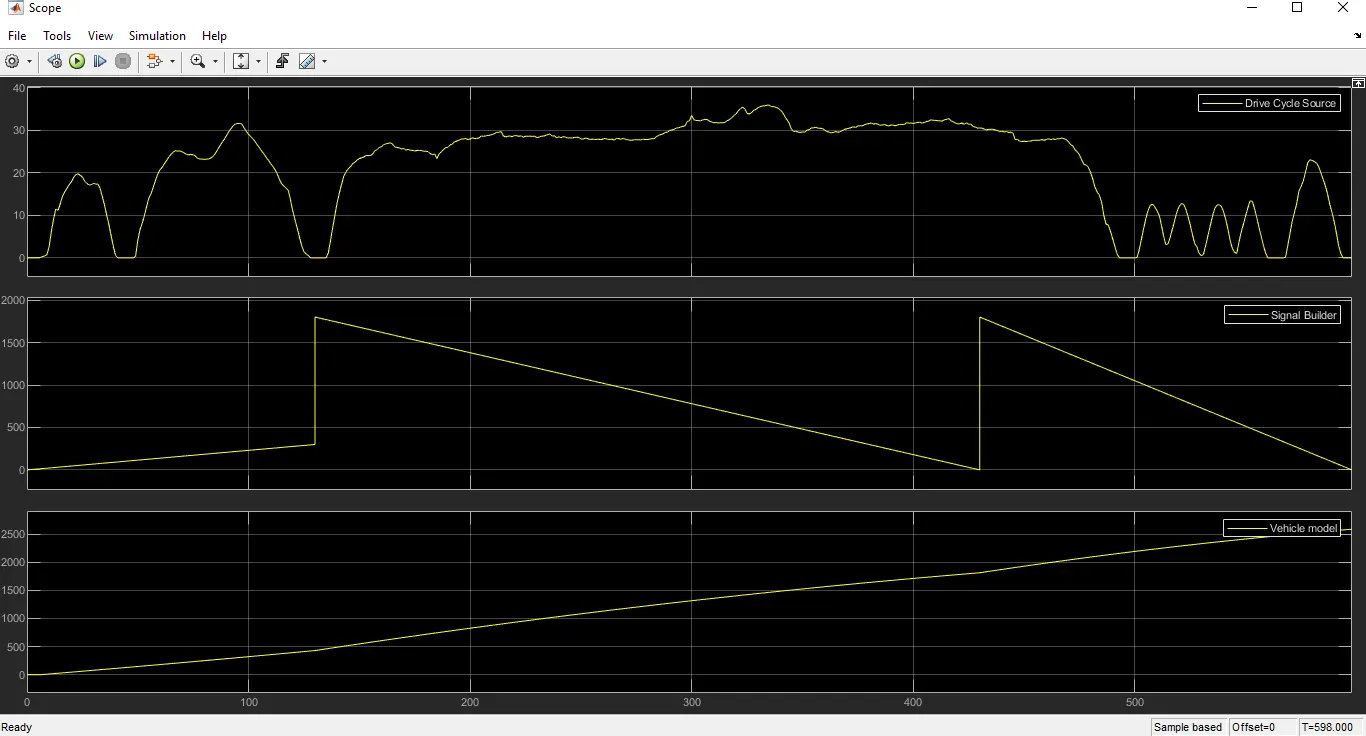
From the result, it can be observed that with velocity changes vehicle speed also changes. According
to increase or decrease in velocity vehicle speed varies.
Conclusion:
Successfully Completed the vehicle model by modeling the remaining equations and simulation stop
time set to 598 sec.