Challenge

Week 7 - Auto ignition using Cantera

KKrishnanand Kushwaha14 Apr 2022

Objective

To plot the variation of Auto-ignition time of methane with a constant Temperature of 1250 K and varying pressure of 1 to 5 atm.
To plot the variation of Auto-ignition time of methane with a constant pressure of 5atm and varying temperature from 950 to 1450 K.
To observe and print the rate of change of molar concentration of the given elements `H_2O,O_2,OH` with respect to the simulation time.
To explain the behavior of the graph for 2 cases
- when Temperature is 1000K and pressure is 5 bar.
- when temperature is 50K and pressure is 5 bar.

Theory:

Auto-ignition temperature

Auto-ignition temperature is the lowest temperature at which ignition starts.

Ignition delay

Ignition delay is the time required for ignition to take place. it depends on temperature, pressure and mixture composition.

Reactor:

A CanteraReactor() represents the simplest form of a chemically reacting system. it corresponds to an extensive thermodynamic control volume V, in which all state variables are homogeneously distributed. The system is generally unsteady, that is, all states are functions of time. in particular, transient state changes due to chemical reactions are possible. However, thermodynamic (but not chemical) equilibrium is assumed to be present throughout the reactor at all instants of time.

Part -I

Case I

For this case the given conditions are

Simulation time 10 sec
fuel: methane(`CH4`)
Temperature 1250K
Pressure varies from 1-5 atm.

Code with explanation

#Importing required libraries

import sys
import numpy as np
import cantera as ct
import matplotlib.pyplot as plt


gas = ct.Solution('gri30.xml')
#define Pressure temperature and time for the simulation
P = np.linspace(1,5,9)
T = 1250
t_start = 0.0
t_end = 10.0
time_step = 1e-3
n = int((t_end - t_start)/time_step)
time_autoI_p = []
states1 = []

#For loop for arying pressure
for i in P:
	gas.TPX = T,i*101325, {'CH4':1,'O2':2,'N2':7.52}
	t_autoI = 0
	T_autoI = 0
	time = 0
	r = ct.IdealGasReactor(gas)
	sim = ct.ReactorNet([r])	
	states = ct.SolutionArray(gas,extra=['time_in_ms','t'])
	print('{:10s} {:10s} {:10s}'.format('t[s]','T[K]','P[Pa]'))
	# for loof for time increment in reactor network
	for n in range(n):
		time += 1e-3
		sim.advance(time)
		states.append(r.thermo.state,time_in_ms = time*1e3,t = time)
		print('{:10.3e} {:10.3f} {:10.3f}'.format(sim.time,r.T,r.thermo.P))
	states1.append(states.T)
	# for loop for appending temperature value for each time step
	for i in range (n):
		T_error = states.T[i] - T - 400
		if T_error > 0:
			T_autoI = states.T[i]
			t_autoI = states.time_in_ms[i]
			break
	time_autoI_p.append(t_autoI)
	#print(states.T)
states1 = np.array(states1)

#Plotting
for k in range(len(P)):
	plt.figure(1)
	plt.plot(states1[k])
	plt.xlabel('number of time steps')
	plt.ylabel('Temperature')
	plt.title('variation of Auto ignition temperature with inlet pressure')
	plt.legend(['1 bar','1.5 bar','2 bar','2.5 bar','3 bar','3.5 bar','4 bar','4.5 bar','5 bar'])
	
plt.figure(2)
plt.plot(P,time_autoI_p,'b-*')
plt.xlabel('Pressure in bar')
plt.ylabel('Auto ignition time[ms]')
plt.title('ignition time delay vs pressure')
plt.show()

Plots

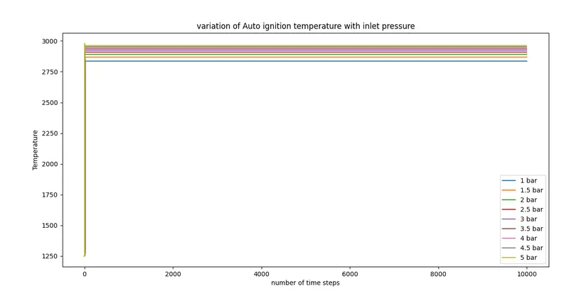
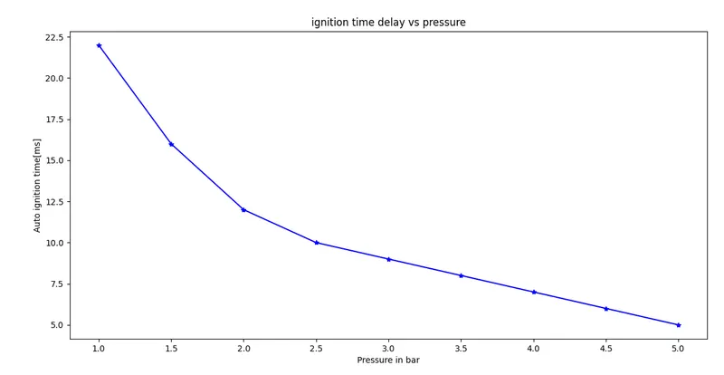
Output table

Initial pressure [atm]	ignition-time delay[seconds]
1	22
1.5	16
2	12
2.5	10
3	9
3.5	8
4	7
4.5	6
5	5

Case II

For this case the given conditions are:

Simulation time 10 sec.
fuel: methane(`CH4`).
Temperature varies from 950 to 1450K.
Pressure 5 atm.

Code with explanation

#Importing required libraries

import sys
import numpy as np
import cantera as ct
import matplotlib.pyplot as plt


gas = ct.Solution('gri30.xml')


#define Pressure temperature and time for the simulation

T = np.linspace(950,1450,11)
t_start = 0.0
t_end = 10.0
time_step = 1e-3
n = int((t_end - t_start)/time_step)
time_autoI_T = []
states1 = []

#For loop for varying Temperature

for i in T:
	gas.TPX = i,5*101325, {'CH4':1,'O2':2,'N2':7.52}
	t_autoI = 0
	T_autoI = 0
	time = 0
	r = ct.IdealGasReactor(gas)
	sim = ct.ReactorNet([r])	
	states = ct.SolutionArray(gas,extra=['time_in_ms','t'])
	print('{:10s} {:10s} {:10s}'.format('t[s]','T[K]','P[Pa]'))
# for loop for appending temperature value for each time step

	for j in range(n):
		time += 1e-3
		sim.advance(time)
		states.append(r.thermo.state,time_in_ms = time*1e3,t = time)
		print('{:10.3e} {:10.3f} {:10.3f}'.format(sim.time,r.T,r.thermo.P))
	states1.append(states.T)
# for loop for appending temperature value for each time step
	for j in range (n):
		T_error = states.T[j] - i - 400
		if T_error > 0:
			T_autoI = states.T[j]
			t_autoI = states.time_in_ms[j]
			break
	time_autoI_T.append(t_autoI)
	
states1 = np.array(states1)

#plotting
for k in range(len(T)):
	plt.figure(1)
	plt.plot(states1[k])
	plt.xlabel('number of time steps')
	plt.ylabel('Temperature')
	plt.title('variation of Auto ignition temperature with inlet pressure')
	plt.legend(['950 K','1000 K', '1050 K','1100 K','1150 K','1200 K','1250 K','1300 K','1350 K','1400 K','1450 K'])
	
plt.figure(2)
plt.plot(T,time_autoI_T,'b-*')
plt.xlabel('Pressure in bar')
plt.ylabel('Auto ignition time[ms]')
plt.title('ignition time delay vs pressure')
plt.show()

Plots

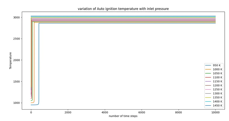
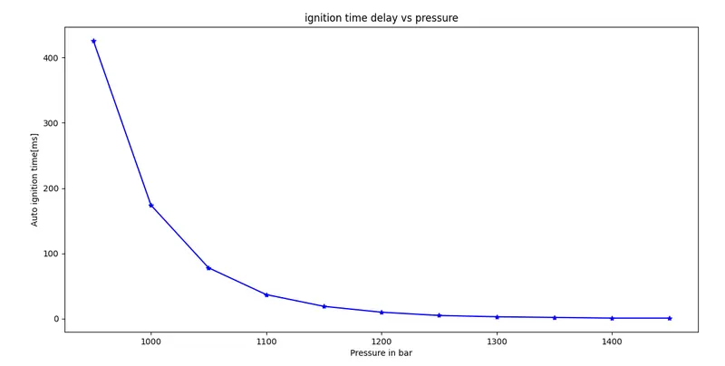
Initial temperature[K]	Ignition delay time[ms]
950	425
1000	175
1050	737
1100	37
1150	21
1200	10
1250	5
1300	3
1400	2
1450	1

Part II

Case I

Python code

#importing necessary libraries
import sys
import numpy as np
import cantera as ct
import matplotlib.pyplot as plt


gas = ct.Solution('gri30.xml')

#defining temperature pressure and mole fraction of species
gas.TPX = 1000,5*ct.one_atm, {'CH4':1,'O2':2,'N2':7.52}
#defining time step
t_start = 0.0
t_end = 10.0
time_step = 1e-3
n = int((t_end - t_start)/time_step)
time = 0
r = ct.IdealGasReactor(gas)
sim = ct.ReactorNet([r])	
time = 0
states = ct.SolutionArray(gas,extra=['time_in_ms','t'])
# for loop for increasing time  and appending all data
for j in range(n):
	time += 1e-3
	sim.advance(time)
	states.append(r.thermo.state,time_in_ms = time*1e3,t = time)


# Plotting
plt.figure(1)
plt.plot(states.time_in_ms,states.X[:,gas.species_index('H2O')])
plt.xlabel('time[ms]')
plt.ylabel('species concentration[H2O]')
plt.figure(2)
plt.plot(states.time_in_ms,states.X[:,gas.species_index('O2')])
plt.xlabel('time[ms]')
plt.ylabel('species concentration[O2]')
plt.figure(3)
plt.plot(states.time_in_ms,states.X[:,gas.species_index('OH')])
plt.xlabel('time[ms]')
plt.ylabel('species concentration[OH]')
plt.show()

Plots for 1000 K

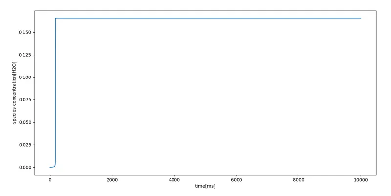
From the graph we can observe that initially the concentration of `H_2O` is zero but it is increasing for a very little time then it becomes constant at 0.16 for rest of the simulation time.

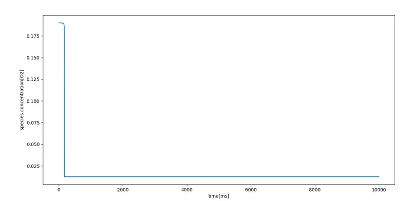
Since `O_2` is a reactant in combustion process. it can be clearly observed that it is suddenly decreasing as combustion starts. and remains constant for the rest of the simulation time.

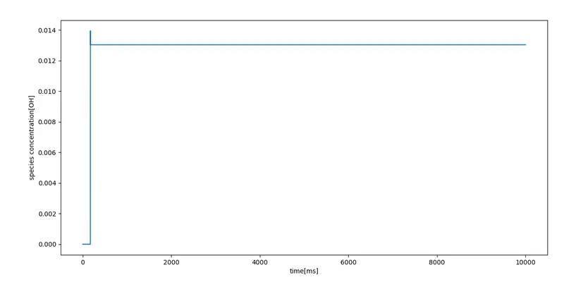
We can observe that the fraction of OH is zero initially but after some time of simulation started OH formed and remains constant for rest of the simulation time. formation of OH is very small as compared to `H_2O`.

Case II

#importing necessary libraries
import sys
import numpy as np
import cantera as ct
import matplotlib.pyplot as plt


gas = ct.Solution('gri30.xml')

#defining temperature pressure and mole fraction of species
gas.TPX = 500,5*ct.one_atm, {'CH4':1,'O2':2,'N2':7.52}
#defining time step
t_start = 0.0
t_end = 10.0
time_step = 1e-3
n = int((t_end - t_start)/time_step)
time = 0
r = ct.IdealGasReactor(gas)
sim = ct.ReactorNet([r])	
time = 0
states = ct.SolutionArray(gas,extra=['time_in_ms','t'])
# for loop for increasing time  and appending all data
for j in range(n):
	time += 1e-3
	sim.advance(time)
	states.append(r.thermo.state,time_in_ms = time*1e3,t = time)


# Plotting
plt.figure(1)
plt.plot(states.time_in_ms,states.X[:,gas.species_index('H2O')])
plt.xlabel('time[ms]')
plt.ylabel('species concentration[H2O]')
plt.figure(2)
plt.plot(states.time_in_ms,states.X[:,gas.species_index('O2')])
plt.xlabel('time[ms]')
plt.ylabel('species concentration[O2]')
plt.figure(3)
plt.plot(states.time_in_ms,states.X[:,gas.species_index('OH')])
plt.xlabel('time[ms]')
plt.ylabel('species concentration[OH]')
plt.show()

Plots for 500 K

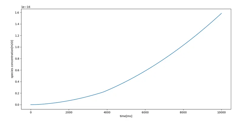
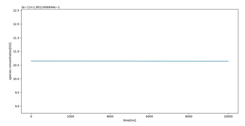
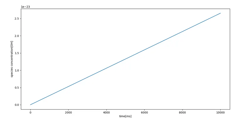
Since we know that methane cannot combust at 500K as its auto-ignition temperature is 873.15 K, combustion does not take place for the given temperature of 500K and this is also evident from the `O_2` plot as its molar concentration does not changes as the time progresses.

But if we look at the graphs of `H_2O` and OH we can observe that their concentration is increasing but the order of increases is not that high, though the combustion has not started still the product is being formed such as `H_2O` and OH, this is because of the ambient reactions that are taking place. The initial temperature and pressure provided are greater than the threshold of these reactions. therefore, we notice a slight increase in the molar concentration of `H_2O` and OH as these ambient reactions are taking place and forming these products even though the combustion has not started.

Week 7 - Auto ignition using Cantera

Ship work like this
in your own course.

Talk to a career counsellor

Ship work like thisin your own course.

Talk to a career counsellor

Ship work like this
in your own course.