Week 5.1 - Mid term project - Solving the steady and unsteady 2D heat conduction problem
The heat equation is a second order partial differential equation that describes how the distribution of some quantity such as heat evolves over time in a solid medium, as it spontaneously flows from place where it is higher towards places where it is lower. It is a special case of the diffusion equation.
For a function `T(x,y,z,t)` of 3 spatial variables `(x,y, z)` and the time variable `t`, the heat equation is
`(∂T)/(∂t)=α*((∂^2 T)/(∂x^2 )+(∂^2 T)/(∂x^2 )+(∂^2 T)/(∂x^2 ))`
Where, alpha (`alpha`) = Thermal diffusivity.
In compact form,
`(∂T)/(∂t)=α*∇^2 T`
his equation describes the flow of heat in homogeneous and isotropic medium, with `T(x,y,z,t)` being the temperature at the point `(x,y,z)` and time `t`.
Informally, the laplacian operator`∇^2` give the difference between the average value of function in the neighbourhood of a point, and its value at the point. Thus, if `T` is the temperature, `∇^2` tells weather (and by how much) the material surrounding is point is hotter or colder on the average, than the material at that point.
The above equation is solved on a 2-D plate which contains four boundaries and the value at those boundaries are:
`T_(bb"left")=400K`
`T_(bb"right")=800K`
`T_(bb"bottom")=900K`
`T_(bb"top")=600K`
The value of thermal diffusivity is taken as 1.4, because more value will give the solution faster.
The assumption made to solve above equation on a 2-D plate are:
- The material is homogeneous and isotropic
- The Alpha is not the function of temperature.
- The radiative and convective losses are neglected.
The final solution is obtained in three ways
- Neglecting unsteady term in the equation (steady state solution).
- Considering unsteady term but solved by explicit method.
- Considering unsteady term but solved by implicit method.
The numerical method used to solve the heat equation for all the above cases is finite difference method. The second order accurate FDM for space term and first order accurate FDM for time term is used to get the solution. So general 2D FDM form of the equation will be;
`(T_i^(n+1)-T_i^n)/(∆t)=α*((T_(i+1,j)-2*T_(i,j)+T_(i-1,j) )/(dx^2 )+(T_(i,j-1)-2*T_(i,j)+T_(I,j+1))/(∆y^2 ))`
The above form will be modified according to the above three cases and the solution will be obtained.
Case I. Solution by neglecting unsteady term.
The FDM form for the steady state equation will be:
`((T_(i+1,j)-2*T_(i,j)+T_(i-1,j) )/(dx^2 )+(T_(i,j-1)-2*T_(i,j)+T_(I,j+1))/(∆y^2 ))=0`
The equation will be solved using Jacobi, Gauss seidel, Successive over relaxation iteration method to check that which method is faster and how it works.
The MATLAB code to solve the above form is
`bb"JACOBI ITERATION"`
clear all
close all
clc
n = 10;%no of grids
L = 1;%domain length
x = linspace(0,L,n);%grid spacing
dx = x(2)-x(1);%grid sizing
y=x;
dy=dx;

T = 300*ones(n,n);% 2D temprature matrix
% boundary conditions
T(:,1) = 400;% left
T(:,n) = 800;% right
T(1,:) = 600;% top
T(n,:) = 900;% bottom
T(1,1) = 500;% top left corner
T(n,1) = 650;% bottom left corner
T(n,n) = 850;% bottom right corner
T(1,n) = 700;% top right corner

error = 1;
tol = 1e-4;
Told = T;

jacobi_iter = 1;

while (error>tol)%convergence loop
    %space loop
    for i = 2:n-1
        for j =2:n-1
            k = 2*((dx^2+dy^2)/(dx^2*dy^2));
            T(i,j) = (1/k)*((Told(i-1,j)+Told(i+1,j))/dx^2+(Told(i,j+1)+Told(i,j-1))/dy^2);
        end
    end
    error = max(max(abs(Told-T)));
    Told = T;
    jacobi_iter = jacobi_iter+1;
end
%plotting
contourf(x,y,T,'showtext','on')
set(gca,'YDIR','reverse')
colorbar
xlabel('Breadth')
ylabel('Length')
title_text = sprintf('total no. of jacobi iteration = %d',jacobi_iter);
title(title_text)
`bb"GAUSS SEIDEL METHOD"`
clear all
close all
clc
n = 10;%no of grids
L = 1;%domain length
x = linspace(0,L,n);%grid spacing
dx = x(2)-x(1);%grid sizing
y=x;
dy=dx;

T = 300*ones(n,n);% 2D temprature matrix
% boundary conditions
T(:,1) = 400;% left
T(:,n) = 800;% right
T(1,:) = 600;% top
T(n,:) = 900;% bottom
T(1,1) = 500;% top left corner
T(n,1) = 650;% bottom left corner
T(n,n) = 850;% bottom right corner
T(1,n) = 700;% top right corner
error = 1;
tol = 1e-4;
Told = T;


GS_iter = 1;
while (error>tol)% convergence loop
  %space loop
    for i = 2:n-1
        for j =2:n-1
            k = 2*((dx^2+dy^2)/(dx^2*dy^2));
            T(i,j) = (1/k)*((T(i-1,j)+Told(i+1,j))/dx^2+(Told(i,j+1)+T(i,j-1))/dy^2);
        end
    end
    error = max(max(abs(Told-T)));
    Told = T;
    GS_iter = GS_iter+1;
end
%plotting
figure(1)
contourf(x,y,T,'showtext','on')
set(gca,'YDIR','reverse')
colorbar
xlabel('Breadth')
ylabel('Length')
title_text1 = sprintf('total no. of GS iteration = %d',GS_iter);
title(title_text1)
`bb"SUCCESSIVE OVER RELAXATION METHOD"`
clear all
close all
clc
n = 10;%no of grids
L = 1;%domain length
x = linspace(0,L,n);%grid spacing
dx = x(2)-x(1);%grid sizing
y=x;
dy=dx;
W = 1.5; %relaxation factor
T = 300*ones(n,n);% 2D temprature matrix
% boundary conditions
T(:,1) = 400;% left
T(:,n) = 800;% right
T(1,:) = 600;% top
T(n,:) = 900;% bottom
T(1,1) = 500;% top left corner
T(n,1) = 650;% bottom left corner
T(n,n) = 850;% bottom right corner
T(1,n) = 700;% top right corner
error = 1;
tol = 1e-4;
Told = T;


SOR_iter = 1;
while (error>tol)%convergence loop
  %space loop
    for i = 2:n-1
        for j =2:n-1
            k = 2*((dx^2+dy^2)/(dx^2*dy^2));
            T(i,j) = (1-W)*Told(i,j)+W*((1/k)*((T(i-1,j)+Told(i+1,j))/dx^2+(Told(i,j+1)+T(i,j-1))/dy^2));
        end
    end
    error = max(max(abs(Told-T)));
    Told = T;
    SOR_iter = SOR_iter+1;
end
% plotting
contourf(x,y,T,'showtext','on')
set(gca,'YDIR','reverse')
colorbar
xlabel('Breadth')
ylabel('Length')
title_text1 = sprintf('total no. of GS iteration = %d',SOR_iter);
title(title_text1)
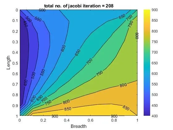
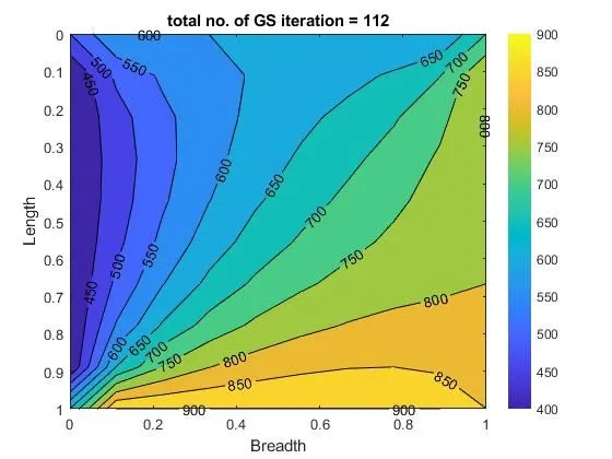
As we are observing the steady temperature distribution in the plate, the final solution with all the method will be visually same, but the number of iterations of each method will be different.
The temperature distribution plot with the number of iterations are;
`bb"OUTPUT PLOT FOR JACOBI ITERATION"`
`bb"OUTPUT PLOT FOR GAUSS SEIDEL ITERATION"`
`bb"OUTPUT PLOT FOR SOR"`
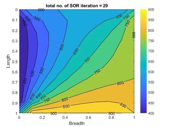
The above graph clearly shows that SOR method takes the smaller number of iterations to converge than the Gauss Seidel and Jacobi. Consequently, d SOR takes less time followed by Gauss Seidel and Jacobi method. To get the solution faster, the successive relaxation factor should be optimum. In above case the relaxation factor from 1-2 to has been tried and the factor 1.5 has given the solution in least number of iterations. There are various formulas are available for optimum relaxation factor but in our case, it has been observed that those are not giving optimum results so, trial and error method is best suitable here to choose the optimum relaxation factor.
As per the error criteria given, the final solution will be the same, but the method to get the solution faster is also equally important. And, SOR is the winner.
Case II. Solution by considering unsteady term (explicit method)
The explicit form of the above equation is easy to form but care should be taken to get the stable solution. The CFL condition based timestep is required to get the stable solution.
the finite difference explicit form of the equation is:
`(T_i^(n+1)-T_i^n)/(∆t)=α*((T_(i+1,j)-2*T_(i,j)+T_(i-1,j) )/(dx^2 )+(T_(i,j-1)-2*T_(i,j)+T_(I,j+1))/(∆y^2 ))`
As the solution for the previous time exist for time marching, this form of the solution is easy to solve. The iterative solvers are not required for this method because system of equations is not getting form. The RHS of the equation is completely known and there is only one unknown in the equation. so, the simple and sort code for this method is,
`bb"MATLAB CODE FOR TRANSIENT EXPLICIT SOLUTION"`
clear all
close all
clc
n = 10;%no of grids
L = 1;%domain length
x = linspace(0,L,n);%grid spacing
y = linspace(0,L,n);%grid spacing
dx = x(2)-x(1);%grid sizing

dy = y(2)-y(1);
% Timesteps
t = 4;
dt = 0.001;
nt = t/dt;
a = 1.4;% Thermal difusivity
T = 300*ones(n,n);% 2D temprature matrix
% boundary conditions
T(:,1) = 400;% left
T(:,n) = 800;% right
T(1,:) = 600;% top
T(n,:) = 900;% bottom
T(1,1) = 500;% top left corner
T(n,1) = 650;% bottom left corner
T(n,n) = 850;% bottom right corner
T(1,n) = 700;% top right corner
Told = T;


for nt = 1:1500 %time loop
    %Space loop
    for i = 2:n-1
        for j =2:n-1
            k1 = (a*dt)/(dx^2);
            k2 = (a*dt)/(dy^2);
            H = (Told(i-1,j)-2*T(i,j)+T(i+1,j));
            V = (Told(i,j+1)-2*T(i,j)+T(i,j-1));
            T(i,j) = Told(i,j)+k1*H+k2*V;
        end
    end
    Told = T;
end
% Plotting
contourf(x,y,T,'showtext','on')
colorbar
set(gca,'YDIR','reverse')
xlabel('Breadth')
ylabel('Length')
title('Temprature field for explicit transient solution')
`bb"OUTPUT PLOT FOR TRANSIENT EXPLICIT SOLUTION"`
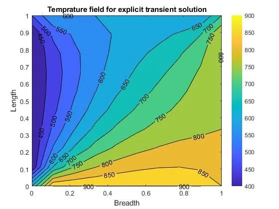
The care should be taken while choosing the timestep for this method. The CFL criteria is considered while choosing timestep which states that,
`(2α*∆t)/(min(∆x^2,∆y^2))≤C`
Where, `C` is courant number and value for `C ` is 0.5 for 2-D heat equation
The above formula will give the time step of 0.0018 and takes the least time to get the stable accurate solution. the decreasing timestep below this value will also give stable accurate solution but the time required to get the solution will be increased. So, we can say that CFL based time step is optimum time step for the explicit method.
Case III. Solution by considering unsteady term (Implicit method)
The implicit method is unconditionally stable but it is difficult and time consuming. Application of implicit method on each node will form a system of linear equations and it needs to be solved by iterative methods. The iterative methods are discussed in the steady state solution and to maintain the consistency, same methods are used in this method.
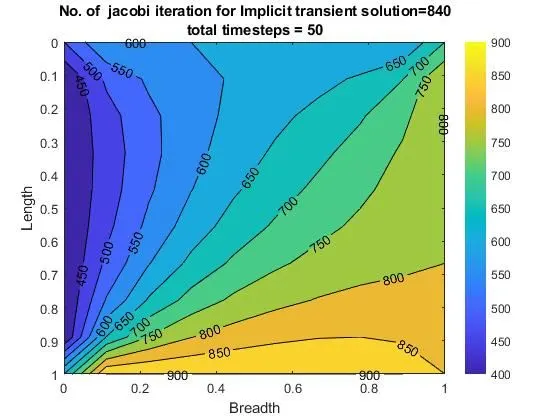
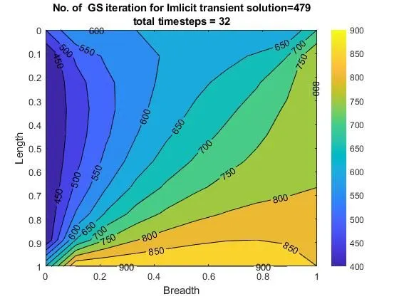
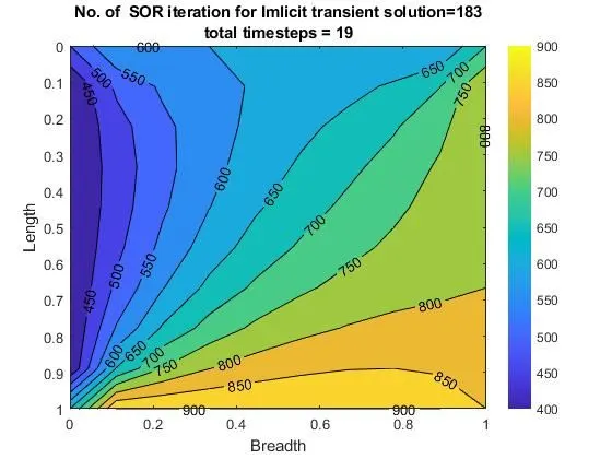
The results of 3 methods are also observed to be same as before, in which SOR will take least iterations followed by Gauss Seidel and Jacobi.
The CFL criteria is not required to be checked for calculating timestep. But, choosing the higher time step can lead to wrong solution. The time step of 0.1 s is closed and solution is solved till sufficient error criteria is achieved. The simulation has not been running for fixed total time, because that will not allow us to get the solution faster. The total iterations and total number of time steps are calculated and compared for all the three methods.
The code to solve the 2D heat equation by implicit method is,
clear all
close all
clc
n = 10;% no. of grids
L = 1; %domain length
x = linspace(0,L,n);% grid spacing
dx = x(2)-x(1);% grid size
y = x;
dy = dx;

% Boundary conditions
T = 400*ones(n,n);% 2-D temprature matrix
T(:,1) = 400;% left
T(:,n) = 800;% right
T(1,:) = 600;% top
T(n,:) = 900;% bottom
T(1,1) = 500;% top left corner
T(n,1) = 650;% bottom left corner
T(n,n) = 850;% bottom right corner
T(1,n) = 700;% top right corner
Told = T;
error = 1;
% time steps
t = 40; %time in seconds
dt = 0.1; %time step size
nt = t/dt; % no. of time steps
a = 1.4; % thermal difusivity
%constant terms
k1 = (a*dt)/(dx^2);
k2 = (a*dt)/(dy^2);
term1 = 1/(1+2*k1+2*k2);
term2 = k1*term1;
term3 = k2*term1;
Tprev = T;
tol = 1e-4; %tolerance
% Iterative solver selection
Iterative_solver = input('Iterative_solver(1. jacobi 2. gauss seidel 3. SOR) =' );

%jacobi method

if Iterative_solver ==1

jacobi_iter = 1;
jacobi_total_timestep = 1;
%time loop
    for z = 1:nt
        error = 100;
    %convergence loop
        while (error>tol)
        %space loop
            for i = 2:n-1
                for j =2:n-1

                H = (Told(i-1,j)+Told(i+1,j));
                V = (Told(i,j-1)+Told(i,j+1));
                T(i,j) = term1*Tprev(i,j)+term2*H+term3*V;
                end
            end
            error = max(max(abs(Told-T)));
            Told = T;

            jacobi_iter = jacobi_iter+1;

        end


    contourf(x,y,T,'showtext','on')
    set(gca,'YDIR','reverse')
    colorbar;
    xlabel('Breadth')
    ylabel('Length')
    title_text1 = sprintf('No. of  jacobi iteration for Implicit transient solution=%d',jacobi_iter);
    title_text2 = sprintf('total timesteps = %d',jacobi_total_timestep);
    title({title_text1,title_text2});
    pause(0.05)
    jacobi_total_timestep = jacobi_total_timestep+1;

        if(T-Tprev < 1e-5)
             break
        end
     Tprev = T;
    end
end

%Gauss Seidel Method

if Iterative_solver ==2

GS_iter = 1;
GS_iter_timestep = 1;
%time loop
    for z = 1:nt
        error = 100;
    %convergence loop
        while (error>tol)
        %space loop
            for i = 2:n-1
                for j =2:n-1

                     H = (T(i,j+1)+T(i,j-1));
                     V = (T(i+1,j)+T(i-1,j));
                     T(i,j) = term1*Tprev(i,j)+term2*H+term3*V;
                end
            end
                 error = max(max(abs(Told-T)));
                 Told = T;

                 GS_iter = GS_iter+1;

        end


    contourf(x,y,T,'showtext','on')
    set(gca,'YDIR','reverse')
    colorbar;
    xlabel('Breadth')
    ylabel('Length')
    title_text1 = sprintf('No. of  GS iteration for Imlicit transient solution=%d',GS_iter);
    title_text2 = sprintf('total timesteps = %d',GS_iter_timestep);
    title({title_text1,title_text2});
    pause(0.05)
    GS_iter_timestep = GS_iter_timestep+1;

         if(T-Tprev < 1e-5)
            break

         end
             Tprev = T;
   end
end

%SOR Method

if Iterative_solver ==3

SOR_iter = 1;
SOR_iter_timestep = 1;
w = 1.5;
%time loop
    for z = 1:nt
        error = 100;
    %convergence loop
        while (error>tol)
        %space loop
            for i = 2:n-1
                for j =2:n-1

                H = (T(i-1,j)+T(i+1,j));
                V = (T(i,j+1)+T(i,j-1));
                T(i,j) = ((1-w)*Told(i,j))+w*(term1*Tprev(i,j)+term2*H+term3*V);
                end
            end
            error = max(max(abs(Told-T)));
            Told = T;

            SOR_iter = SOR_iter+1;

        end


    contourf(x,y,T,'showtext','on')
    set(gca,'YDIR','reverse')
    colorbar;
    xlabel('Breadth')
    ylabel('Length')
    title_text1 = sprintf('No. of  SOR iteration for Imlicit transient solution=%d',SOR_iter);
    title_text2 = sprintf('total timesteps = %d',SOR_iter_timestep);
    title({title_text1,title_text2});
    pause(0.05)
    SOR_iter_timestep = SOR_iter_timestep+1;

    if(T-Tprev < 1e-5)
        break

    end
    Tprev = T;
    end
end
The results with all the three methods obtained are:
Discussion
- As all cases are observed for final steady solution, the temperature plots are same.
- The SOR method is better to get the solution faster compared to Gauss Seidel and Jacobi.
- The explicit method is easy to form, but stability needs to be checked with CFL.
- The implicit method needs iterative solver, where explicit gives the direct solution.
- Implicit methods are difficult to form but stability make it an attractive choice.
- The CFL best time step is selected in the explicit method to get the stable solution.
- The successive over-relaxation parameter is selected based on trial and error method, because the formulas available in literature are not reliable.