Week 7 - Simulation of a 1D Super-sonic nozzle flow simulation using Macormack Method

Objective: - To simulate the isentropic flow through a quasi 1D subsonic-supersonic nozzle using both the conservative and non- conservative Forms of the governing equations and solve them using the McCormack’s technique and comparing their solutions.

Description: We consider the study, isentropic flow through a convergent divergent nozzle. the flow at the inlet to the nozzle comes from reservoir. the cross-section area of the reservoir is very large and hence velocity is very small the flow is locally subsonic the convergent section of the nozzle. Sonic at the throat and supersonic at the divergent.

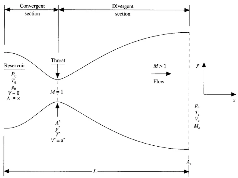
Let us consider a small control volume of the nozzle as shown below.

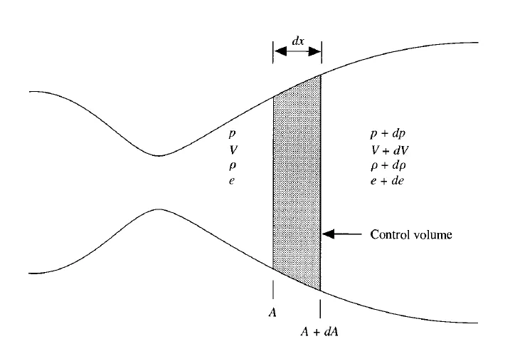
We assume that at a given section, where the cross-section area is A, the flow properties are uniform across the section. Hence, although the area of the nozzle changes as a function of distance along the nozzle `X`and therefore in reality the flow field is two dimensional (the flow where is in the two-dimensional `X-Y` space), we make the assumption that the flow properties very only with `X`; this is tantamount to assuming uniform flow properties across any given cross-section. Such flow is defined as Quasi one-dimensional flow.

The governing continuity momentum and energy equation in terms of non-dimensional variables for the quasi-one-dimensional study and isentropic flow can be expressed respectively as:

Non-Conservative continuity equation

`(∂ρ^')/(∂t^' )=-ρ^' ((∂V^')/(∂x^' ))-ρ^' V^' ((∂(l n⁡A^'))/(∂x^' )) V^' ((∂ρ^')/(∂x^' ))`

Non-Conservative momentum equation:

`(∂V^')/(∂t^' )=-V^' ((∂V^')/(∂x^' ))-(1/γ)((∂T^')/(∂x^' )+T^'/P^' ((∂ρ)/(∂x^' )))`

Non-Conservative energy equation:

`(∂T^')/(∂x^' )=-V^' ((∂T^')/(∂x^' ))-(γ-1) T^' [(∂V^')/(∂x^' )+V^' (∂(ln A^' ))/(∂x^' )]`

Conservative Continuity equation:

`(∂(ρ^' A^'))/(∂t^' )+(∂(ρ^' A^' V^'))/(∂x^' )=0`

Conservative momentum equation:

`(∂(ρ^' A^' V^'))/(∂t^' )+(∂[ρ^' (V^' )^2+(1/γ) ρ^' A^' ])/(∂x^' )=(1/γ) ρ^' ((∂A^')/(∂x^' ))`

Conservative energy equation

`(∂[ρ^' (e^'/(γ-1)+(γ/2) (V^' )^2 ) A^' ])/(∂t^' )+(∂[ρ^' (e^'/(γ-1)+(γ/2) (V^' )^2 ) V^' A^'+ρ^' A^' V^' ])/(∂x^' )=0`

For air at standard conditions, 𝛄 = 1.4

These equations are solved by McCormack method using time marking process

McCormack Method:

Let f(x) is the equation to be solve using this method, then the following steps are used:

Initial profile

Before the calculation, the initial profile for all the flow field variables which are velocity, density and temperature has to be determined. these are guess values but should be specified with more awareness on the problem.

Predictor method

`((∂f)/(∂t))_p=(f(i+1)-f(i))/(∆x)`

Solution update

`f_p=f_text(initial)+([∂f]/[∂t])_p*∆t`

`f_p=text(flow field variables calculated after the predictor step)`

`f_text(initial)=text(flow field variable in the initial step)`

`∆t=text[time step size]`

Corrector step

`((∂f_p)/(∂t))_c=(f(i)-f(i-1))/(∆x)`

`((∂f)/(∂t))_c=0.5(((∂f)/(∂t))_p+((∂f_p)/(∂t))_c)`

Final solution update

`f_text(sol)=f_text(initial)+((∂f)/(∂t))_text(avg)*∆t`

`f_text(sol)=text(final solution of the flow field variable for the first time step)`

MATLAB CODE WITH EXPLAINATION

function code for conservative method

function [rho_c,p_c,t_c,v_c,mass_flow_rate_c,mass_flow_rate_th_c] = conservative_one_D(n,x,dx,a,nt,gamma,th)
%calculating initial values
    for i = 1:length(x)
        if x(i)>=0 && x(i)<=0.5
            rho_c(i) = 1;
            t(i) = 1;

        elseif x(i)>=0.5 && x(i)<=1.5
            rho_c(i) = 1-0.366*(x(i)-0.5);
            t(i) = 1-0.167*(x(i)-0.5);

        elseif x(i)>=1.5 && x(i)<=3.0
            rho_c(i) = 0.634-0.3879*(x(i)-1.5);
            t(i) = 0.833-0.3507*(x(i)-1.5);

        end
    end
    %defining variables
    v_c = 0.59./(rho_c.*a);   %Velocity

    p = rho_c.*t;%pressure
    % defining solution vectors
    u1 = rho_c.*a;   
    u2 = rho_c.*a.*v_c;
    u3 = rho_c.*((t/(gamma-1))+(gamma/2)*v_c.^2).*a;

   
    c = 0.5; %courant no.
    dt = min(c.*(dx./(sqrt(t)+v_c))); 
    %time loop
    for k = 1:nt
    
        rho_old = rho_c;
        v_old = v_c;
        t_old = t;
        p_old = p;
        u1_old = u1;
        u2_old = u2;
        u3_old = u3;
        % flux terms
        f1 = u2;
        f2 = (u2.^2./u1)+((gamma-1)/gamma)*(u3-(gamma/2)*u2.^2./u1);
        f3 = gamma.*((u2.*u3)./u1)-(gamma*(gamma-1)/2).*(u2.^3./u1.^2);

        % predictor method
            for j = 2:n-1                 
                j2(j)= (1/gamma).*rho_c(j).*t(j).*((a(j+1)-a(j))/dx);
        %   continuityequation          
                du1dt_p(j) = -(f1(j+1)-f1(j))/dx;
        %   momentum equation              
                du2dt_p(j) = -((f2(j+1)-f2(j))/dx)+j2(j);
        %   energy equation              
                du3dt_p(j) = -(f3(j+1)-f3(j))/dx;

                %solution update
                u1(j) = u1(j)+du1dt_p(j).*dt;
                u2(j) = u2(j)+du2dt_p(j).*dt;
                u3(j) = u3(j)+du3dt_p(j).*dt;

                %updating premitive variables
                rho_c(j) = u1(j)./a(j);
                v_c(j) = u2(j)./u1(j);
                t(j) = (gamma-1)*((u3(j)./u1(j))-((gamma/2).*v_c(j).^2));
                p(j)=rho_c(j).*t(j);
                %updating flux vectors
                f1(j) = u2(j);
                f2(j) = (u2(j).^2./u1(j))+((gamma-1)/gamma)*(u3(j)-(gamma/2)*u2(j).^2./u1(j));
                f3(j) = gamma.*((u2(j).*u3(j))./u1(j))-(gamma*(gamma-1)/2).*(u2(j).^3./u1(j).^2);

            end
            
    % corrector method
            for j = 2:n-1      
                j2(j)= (1/gamma).*rho_c(j).*t(j).*((a(j)-a(j-1))/dx);
        %   continuity equation              
                du1dt_c(j) = -(f1(j)-f1(j-1))/dx;
        %   momentum equation              
                du2dt_c(j) = -((f2(j)-f2(j-1))/dx)+j2(j);
        %   energy equation              
                du3dt_c(j) = -(f3(j)-f3(j-1))/dx;

            end

        % computing average time derivation 
                du1dta = 0.5*(du1dt_p+du1dt_c);
                du2dta = 0.5*(du2dt_p+du2dt_c);
                du3dta = 0.5*(du3dt_p+du3dt_c);


         %final solution update
                for i =2:n-1
                    u1(i) = u1_old(i)+du1dta(i)*dt;
                    u2(i) = u2_old(i)+du2dta(i)*dt;
                    u3(i) = u3_old(i)+du3dta(i)*dt;

                end

    % Boundary conditions
        % inlet
            u1(1) = rho_c(1).*a(1);
            u2(1) = 2*u2(2)-u2(3);
            u3(1) = u1(1).*((t(1)./(gamma-1)+(gamma/2).*v_c(1).^2));

        % outlet
            u1(n) = 2*u1(n-1)-u1(n-2);
            u2(n) = 2*u2(n-1)-u2(n-2);
            u3(n) = 2*u3(n-1)-u3(n-2);

        % updating premitive variables
            rho_c = u1./a;
            v_c = u2./u1;
            t_c = (gamma-1)*((u3./u1)-((gamma/2).*v_c.^2));
            p_c = rho_c.*t_c;
            mach_no = v_c./sqrt(t_c);
            mass_flow_rate_c = rho_c.*a.*v_c;
            
            
        %calculating values at throat
            p_th(k) = p(th);
            mach_no_th(k) = mach_no(th);
            rho_th(k) = rho_c(16);
            t_th(k)=t(16);
            mass_flow_rate_th_c(k) = mass_flow_rate_c(th);
        % plotting non dimensional distance through nozzle vs non dimensional mass flow rate at 4 different timesteps
            if k==1
                figure(3)
                plot(x,mass_flow_rate_c)
                hold on
            elseif k==100
                figure(3)
                plot(x,mass_flow_rate_c)
                hold on
            elseif k==200
                figure(3)
                plot(x,mass_flow_rate_c)
                hold on
            elseif k==700
                figure(3)
                plot(x,mass_flow_rate_c)
                hold on
                xlabel('non dimensional distance through nozzle')
                ylabel('non dimensional mass flow rate')
                legend('timestep = 0','timestep = 100','timestep = 200','timestep = 700')
                hold on
                sgtitle('non dimensional distance through nozzle vs non dimensional mass flow rate at 4 different timesteps')
            end
    end
%plotting  non dimensional distance through nozzle vs premitive variavles
    figure(1)
    subplot(4,1,1)
    plot(x,rho_c,'b','linewidth',2)
    xlabel('non dimensional distance through nozzle')
    ylabel('density')
    grid on
    subplot(4,1,2)
    plot(x,v_c,'r','linewidth',2)
    xlabel('non dimensional distance through nozzle')
    ylabel('velocity')
    grid on
    subplot(4,1,3)
    plot(x,t,'g','linewidth',2)
    xlabel('non dimensional distance through nozzle')
    ylabel('temprature')
    grid on
    subplot(4,1,4)
    plot(x,p,'y','linewidth',2)
    xlabel('non dimensional distance through nozzle')
    ylabel('pressure')
    grid on
    sgtitle('non dimensional distance through nozzle vs premitive variavles')
%plotting variables at throat against time step 
    figure(2)
    subplot(4,1,1)
    plot(mach_no_th,'color','r')
    xlabel('no. of timesteps')
    ylabel('mach number')
    grid on
    subplot(4,1,2)
    plot(p_th,'color','y')
    xlabel('no. of timesteps')
    ylabel('non-dimensional pressure')
    grid on
    subplot(4,1,3)
    plot(rho_th,'color','b')
    xlabel('no. of timesteps')
    ylabel('non-dimensional density')
    grid on
    subplot(4,1,4)
    plot(mass_flow_rate_th_c,'color','g')
    xlabel('no. of timesteps')
    ylabel('mass flow rate')
    grid on
    
    
    pause(0.0003)
end

 

function code for non-conservative method

function [rho,p,t,v,mass_flow_rate,mass_flow_rate_th] = non_conservative_one_d(n,c,x,dx,gamma,a,nt,th)   
    % claculating initial profile 
    rho = 1-0.3146*x;%density
    t = 1-0.2314*x;%temprature
    v = (0.1+1.09*x).*t.^0.5;%velocity
    dt=min(c.*dx./(sqrt(t)+v));
    % time loop
    for k = 1:nt
       rho_old = rho;
        v_old = v;
        t_old = t;
    %     predictor method

        for j = 2:n-1           
            dvdx(j) = (v(j+1)-v(j))/dx;
            drhodx(j) = (rho(j+1)-rho(j))/dx;
            dtdx(j) = (t(j+1)-t(j))/dx;
            d_log_a_dx(j) = (log(a(j+1))-log(a(j)))/dx;
    %         continuity equation
            drhodt_p(j) = -rho(j)*dvdx(j)-rho(j)*v(j)*d_log_a_dx(j)-v(j)*drhodx(j);
    %         momentum equation
            dvdt_p(j) = -v(j)*dvdx(j)-(1/gamma)*(dtdx(j)+(t(j)/rho(j))*drhodx(j));
    %         energy equation
            dtdt_p(j) = -v(j)*dtdx(j)-(gamma-1)*t(j)*(dvdx(j)+v(j)*d_log_a_dx(j));
    %         solution update
               rho(j) = rho(j)+drhodt_p(j)*dt;
               v(j) = v(j)+dvdt_p(j)*dt;         
               t(j) = t(j)+dtdt_p(j)*dt;

        end
    %        corrector method

        for j = 2:n-1  
            dvdx(j) = (v(j)-v(j-1))/dx;
            drhodx(j) = (rho(j)-rho(j-1))/dx;
            dtdx(j) = (t(j)-t(j-1))/dx;
            d_log_a_dx(j) = (log(a(j))-log(a(j-1)))/dx;
%         continuity equation
            drhodt_c(j) = -rho(j)*dvdx(j)-rho(j)*v(j)*d_log_a_dx(j)-v(j)*drhodx(j);
%         momentum equation
            dvdt_c(j) = -v(j)*dvdx(j)-(1/gamma)*(dtdx(j)+(t(j)/rho(j))*drhodx(j));
%         energy equation
            dtdt_c(j) = -v(j)*dtdx(j)-(gamma-1)*t(j)*(dvdx(j)+v(j)*d_log_a_dx(j));

        end

    %      compute the average time derivative   
            dvdt = 0.5*(dvdt_p+dvdt_c);
            drhodt = 0.5*(drhodt_p+drhodt_c);
            dtdt = 0.5*(dtdt_p+dtdt_c);
    %         final soluton update
            for i = 2:n-1
            rho(i) = rho_old(i)+drhodt(i)*dt;
            v(i) = v_old(i)+dvdt(i)*dt;
            t(i) = t_old(i)+dtdt(i)*dt;
            end
    %     apply the boundary condition
        % inlet
        v(1) = 2*v(2)-v(3);
        % outlet
        v(n) = 2*v(n-1)-v(n-2);
        rho(n) = 2*rho(n-1)-rho(n-2);
        t(n) = 2*t(n-1)-t(n-2);   
    % updating premitive variables
        p = rho.*t;
        mach_no = v./sqrt(t);
        mass_flow_rate = rho.*a.*v;
        
    

        %calculating values at throat
        p_th(k) = p(th);
        mach_no_th(k) = mach_no(th);
        rho_th(k) = rho(16);
        mass_flow_rate_th(k) = mass_flow_rate(th);
%        plotting  non dimensional distance through nozzle vs non dimensional mass flow rate at 6 different timesteps
        if k ==1
            figure(6)
            plot(x,mass_flow_rate)
           
%             legend('timestep = 0')
            hold on
        elseif k==50
            figure(6)
            plot(x,mass_flow_rate)
          
%             legend('timestep = 50')
            hold on
        elseif k==100
            figure(6)
            plot(x,mass_flow_rate)
          
%             legend('timestep = 100')
            hold on
        elseif k==150
            figure(6)
            plot(x,mass_flow_rate)            
           
%             legend('timestep = 150')
            hold on
        elseif k==200
            figure(6)
            plot(x,mass_flow_rate)
            
%             legend('timestep = 200')
            hold on
        elseif  k==700
            figure(6)
            plot(x,mass_flow_rate)          
            xlabel('non-dimensional distane through nozzle')
            ylabel('non-dimensional mass flow rate')
            hold on
            
            legend('timestep = 0','timestep = 50','timestep = 100','timestep = 150','timestep = 200','timestep = 700')
            title('non dimensional distance through nozzle vs non dimensional mass flow rate at 6 different timesteps')
            hold on
        end
    end
    
%     plotting  non dimensional distance through nozzle vs premitive variavles
    figure(4)
        subplot(4,1,1)
            plot(x,v,'y','linewidth',2) 
            xlabel('non dimensional distance through nozzle')
            ylabel('velocity')
            grid on
        subplot(4,1,2)
           plot(x,t,'g','linewidth',2)
           xlabel('non dimensional distance through nozzle')
           ylabel('temprature')
           grid on
        subplot(4,1,3)
           plot(x,rho,'r','linewidth',2)
           xlabel('non dimensional distance through nozzle')
           ylabel('density')
           grid on
        subplot(4,1,4)
           plot(x,p,'b','linewidth',2)
           xlabel('non dimensional distance through nozzle')
           ylabel('pressure')
           grid on
            sgtitle('non dimensional distance through nozzle vs premitive variables')
            
% plotting variables at throat against time step             
   figure(5)   
        subplot(4,1,1)
            plot(mach_no_th,'color','r')
            ylabel('mach number')
            xlabel('no. of timesteps')
            grid on
        subplot(4,1,2)
            plot(p_th,'color','y')
            ylabel('non-dimensional pressure')
            xlabel('no. of timesteps')
            grid on
        subplot(4,1,3)
            plot(rho_th,'color','b')
            ylabel('non-dimensional density')
            xlabel('no. of timesteps')
            grid on
        subplot(4,1,4)
            plot(mass_flow_rate_th,'color','g')
            ylabel('non dimensional mass flow rate')
            xlabel('no. of timesteps')
            grid on
            pause(0.0003)
       
end

Main code

clear all
close all
clc
n = 31;%no. of grids
x = linspace(0,3,n);%grid spacing
dx = x(2)-x(1);%grid size
a = 1+2.2*(x-1.5).^2;%area
gamma = 1.4;
c = 0.5;%courant no.
nt = 1400;%no. of time steps
th = (n+1)/2;  %index no. for throat 
%function calling for conservative 
   [rho_c,p_c,t_c,v_c,mass_flow_rate_c,mass_flow_rate_th_c] = conservative_one_D(n,x,dx,a,nt,gamma,th);
%fnction calling for non-conservative
   [rho,p,t,v,mass_flow_rate,mass_flow_rate_th] = non_conservative_one_d(n,c,x,dx,gamma,a,nt,th);
% plotting normalized mass flow rate for conservative vs non-conservative
figure(7)
plot(x,mass_flow_rate_c)
hold on
plot(x,mass_flow_rate)
xlabel('non-dimensional distance through nozzle')
ylabel('non-dimensional mass flow rate')
legend('conservative','non-conservative')
title('normalized mass flow rate for conservative vs non-conservative')

FOR 31 GRIDS

OUTPUT PLOT FOR CONSERVATIVE METHOD

figure(1)

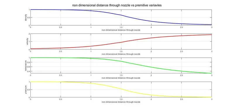
The above plot shows the variation of premitive variables along the nozzle length, here density, temperature and pressure is decreasing along the nozzle length but velocity is increasing along the length.

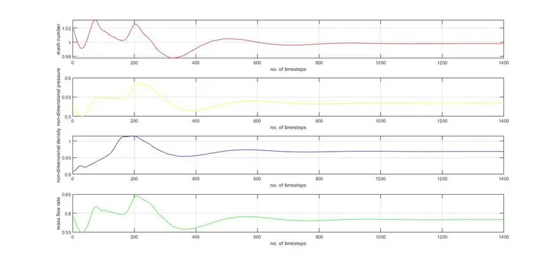
figure(2)

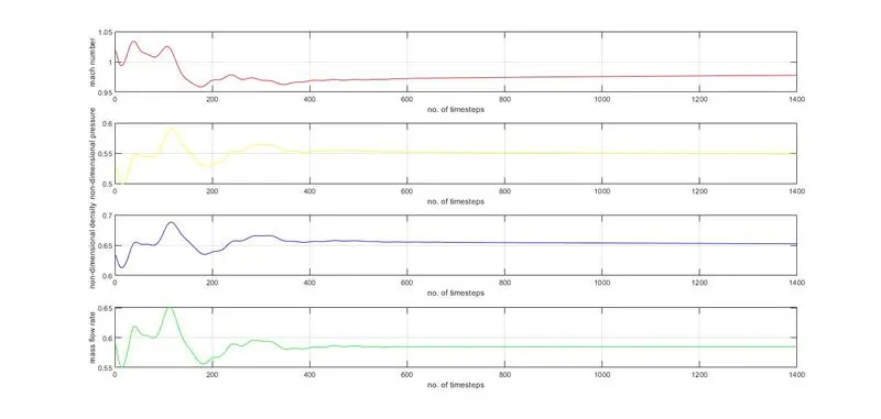
the above figure shows the variation of different premitive variables at throat with the timestep, here mack no. is changing slightly upto 600 timestep then after it is showing constant value. and similar behavior is also shown by other variables e.g, pressure, density and mass flow rate(non-dimensional).

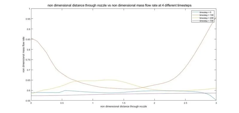
Figure(3)

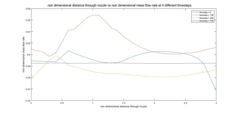
the above plot shows the variation of mass flow distribution through the nozzle at different times during the time marching process.

OUTPUT PLOT FOR NON-CONSERVATIVE METHOD

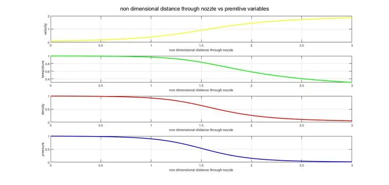
Figure(4)

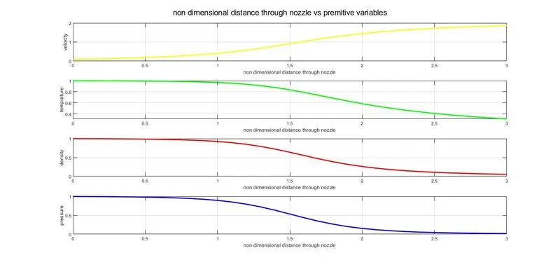
The above plot shows the variation of premitive variables along the nozzle length, here density, temperature and pressure is decreasing along the nozzle length but velocity is increasing along the length.

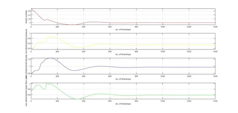
Figure(5)

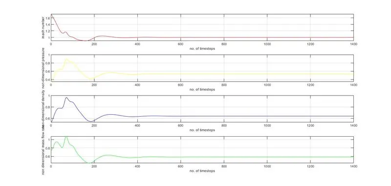
the above figure shows the variation of different premitive variables at throat with the timestep, here mack no. is changing slightly upto 400 timestep then after it is showing constant value. and similar behavior is also shown by other variables e.g, pressure, density and mass flow rate(non-dimensional).

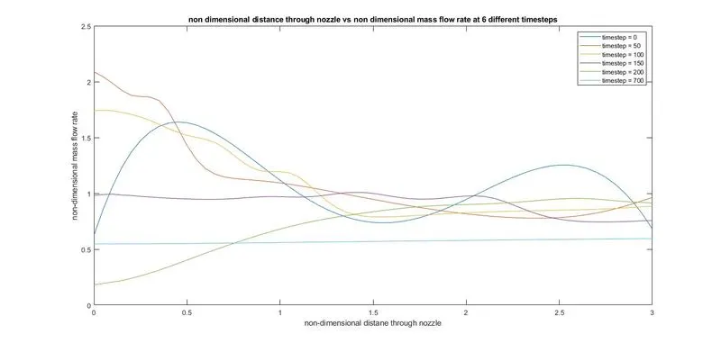
Figure(6)

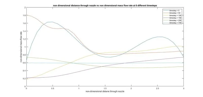
the above plot shows the variation of mass flow distribution through the nozzle at different times during the time marching process.

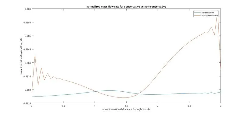
Figure(7)

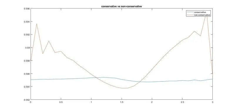
the above plot shows the comparative distribution of mass flow rate in conservative and non conservative form.

FOR 61 GRIDS

OUTPUT PLOT FOR CONSERVATIVE METHOD

figure(1)

figure(2)

figure(3)

figure(4)

figure(5)

figure(6)

figure(7)

Grid independence test and comparing the final result

values at throat node at last time step

	`rho^'`	`temp^'`	`P^'`	M
exact soltion	0.634	0.833	0.528	1
conservative (n=31)	0.6525	0.8411	0.5488	0.9777
non-conservative (n=31)	0.6387	0.8365	0.5342	0.9994
non-conservative (n=61)	0.0527	0.3079	0.0162	0.9979

the above table shows that the program written is independent of grid points in mesh. also it can be seen the the non-conservative solution give more accurate solution than the conservative solution. this happens because the residual that remain after each time step are reduced faster in non-conservative form. At last time step the residual was `10^(-6)` in non-conservative form and was `10^(-3)` in conservative form.