Week 3.5 - Deriving 4th order approximation of a 2nd order derivative using Taylor Table method

Objective

• to derive the `4^(th)`order approximation scheme of the second-order derivative.

1. Central differencing
2. Skewed right-sided difference
3. Skewed left-sided difference

• To write a program in MATLAB to evaluate the second-order derivative of the analytical function, i.e., and compare with the 3 numerical approximations derive earlier.
• Using a plot, compare the absolute error with respect to above-mentioned scheme.
• Compare above-mentioned scheme with forward and backword differencing approximation scheme.
• The usefulness of the skewed scheme over the central differencing scheme.

Taylor’s expansion:

`f(x+∆x)=f(x)+∆x*frac[∂f(x)][∂x]+frac[(∆x)^2][2!] frac[∂^2 f(x)][∂x^2 ]+(∆x)^3/(3!) frac(∂^3 f(x))(∂x^3 )+⋯+(∆x)^n/(n!) (∂^n f(x))/(∂x^n )`

Discretization: PDE to Algebraic equation

For deriving the higher-order approximations, it is not as simple to just apply some algebraic operation and get the result but rather it becomes too complex to convert derivative into algebraic equations.

To ease out, we use a handy tool called as ‘Taylor’s table’ to derive: The process starts with assuming a polynomial based on terms i.e., grid points which depends on an order of approximation and derivative. The coefficient of the polynomial are unknowns which are inserted into the Taylor’s table and evaluation done either through simple manipulation or matrix calculation.

`4^(th)`order central difference scheme for the second order derivative

Let us consider 5 grid points including `x` as central grid point.

`(x-2*dx),(x-dx),(x),(x+dx),(x+2*dx)`

Based on selected grid points, a polynomial is assumed shown below

`(d^2 f(x))/(dx^2 )=a*f(x-2*dx)+b*f(x-dx)+c*f(x)+d*f(x+dx)+e*f(x+2*dx)`

Taylor’s table for Central difference scheme

`(d^2 f(x))/(dx^2 )`	`f(x)`	`f'(x)*dx`	`f''(x)*dx^2`	`f'''(x)*dx^3`	`f''''(x)*dx^4`
` a*f(i-2)`	a	-2a	4a/2	-8a/6	16a/24
`b*f(i-2)`	b	-b	b/2	-b/6	b/24
`c*f(i)`	c	0	0	0	0
`d*f(i+1)`	d	d	d/2	d/6	d/24
`e*f(i+2)`	e	2e	4e/2	8e/6	16e/24
∑above terms	0	0	1	0	0

So, on coupling together terms to form equations

`a+b+c+d+e=0`

`-2a-b+d+2e=0`

`(4a)/2+b/2+d/2+(4e)/2=1`

`(-8a)/6-b/6+d/6+(8e)/6=0`

`(16a)/24+b/24+d/24+(16e)/24=0`

By solving these equations in matrix form [AX=B], we can obtain the values of coefficients a, b, c, d, e which can be substituted in above formula to obtain the central difference approximation

`[[1,1,1,1,1],[-2,-1,0,1,2],[4/2,1/2,0,1/2,4/2],[-8/6,-1/6,0,1/6,8/6],[16/24,1/24,0,1/24,16/24]][[a],[b],[c],[d],[e]]=[[0],[0],[1],[0],[0]]`

MATLAB Code for solving the Matrix for values of coefficients

A = [1 1 1 1 1;-2 -1 0 1 2;4/2 1/2 0 1/2 4/2; -8/6 -1/6 0 1/6 8/6;16/24 1/24 0 1/24 16/24]
B = [0;0;1;0;0]
X = inv(A)*B

On solving matrix we get

`X=A^(-1)*B`

`[[a],[b],[c],[d],[e]]=[[-0.0833],[1.3333],[-2.5000],[1.3333],[-0.0833]]`

On substituting the values, we get

`(d^2 f(x))/(dx^2 )=((-0.83333*e^(x-2*dx)*co s⁡(x-2*dx) )+(1.333333*e^(x-dx)*co s⁡(x-dx) )+(-2.50000*e^x*co s⁡(x) )+(1.333333*e^(x+dx)*co s⁡(x+dx) )+(-0.83333*e^(x+2*dx)*co s⁡(x+2*dx) ))/(dx^2 )`

`4^(th)` order skewed right sided difference scheme for the second order derivative

Let us consider 6 grid points including x as leftmost grid point

`(x),(x+dx),(x+2*dx),(x+3*dx)+(x+4*dx),(x+5*dx)`

Based on selected grid points, a polynomial is assumed shown below

`(d^2 f(x))/(dx^2 )=a*f(x)+b*f(x+dx)+c*f(x+2*dx)+d*f(x+3*dx)+e*f(x+4*dx)+g*f(x+5dx)`

Taylor’s table for skewed right sided difference scheme

`(d^2 f(x))/(dx^2 )`	`f(x)`	`f^' (x)*dx`	`f^'' (x)*(dx)^2`	`f^''' (x)*(dx)^3`	`f^(iv) (x)*(dx)^4`	`f^v (x)*dx^5`
`a*f(x)`	a	0	0	0	0	0
`b*f(x+dx)`	b	b	b/2	b/6	b/24	b/120
`c*f(x+2*dx)`	c	2c	4c/2	8c/6	16c/24	32c/120
`d*f(x+3*dx)`	d	3d	9d/2	27d/6	81d/24	243d/120
`e*f(x+4*dx)`	e	4e	16e/2	64e/6	256e/24	1024e/120
`g*f(x+5*dx)`	g	5g	25g/2	125g/6	625g/24	3125g/120
∑above terms	0	0	1	0	0	0

So, on coupling together terms to form equations

`a+b+c+d+e+g=0`

`b+2c+3d+4e+5g=0`

`b/2+(4c)/2+(9d)/2+(16e)/2+(25g)/2=1`

`b/6+(8c)/6+(27d)/6+(64e)/6+(125g)/6=0`

`b/24+(16c)/24+(81d)/24+(256e)/24+(625g)/24=0`

`b/120+(32c)/120+(243d)/120+(1024e)/120+(3125g)/120=0`

By solving these equations in matrix form [AX=B], we can obtain the values of coefficients a, b, c, d, e which can be substituted in above formula to obtain the skewed right sided difference scheme

`[[1,1,1,1,1,1],[0,1,2,3,4,5],[0,1/2,4/2,9/2,16/2,25/2],[0,1/6,8/6,27/6,64/6,125/6],[0,6/24,16/24,81/24,256/24,625/24],[0,1/120,32/120,243/120,1024/120,3125/120]][[a],[b],[c],[d],[e],[g]]=[[0],[0],[1],[0],[0],[0]]`

MATLAB Code for solving the Matrix for values of coefficients

C = [1 1 1 1 1 1;0 1 2 3 4 5;0 1/2 2 9/2 16/2 25/2;0 1/6 8/6 27/6 64/6 125/6;0 1/24 16/24 81/24 256/24 625/24;0 1/120 32/120 243/120 1024/120 3125/120]
D = [0;0;1;0;0;0]
Y = inv(C)*D

On solving matrix we get

`[[a],[b],[c],[d],[e],[g]]=[[3.7500],[-12.8333],[17.8333],[-13.0000],[5.0833],[-0.8333]]`

On substituting the values, we get

`(d^2 f(x))/(dx^2 )=((3.7500*e^x*cos⁡(x)+(-12.8333*e^(x+dx)*cos⁡(x+dx) )+(17.8333*e^(x+2*dx)*cos⁡(x+2*dx))+(-13.0000*e^(x+3*dx)*cos⁡(x+3*dx) 〗 )+(5.0833*e^(x+4*dx)*cos⁡(x+4*dx) )+(-0.8333*e^(x+5*dx)*cos⁡(x+5*dx) ))/dx^2`

order skewed left sided difference scheme for the second order derivative

Let us consider 6 grid points including i as rightmost grid point

`(i-5*dx),(i-4*dx),(i-3*dx),(i-2*dx),(i-dx),(i),`

Based on selected grid points, a polynomial is assumed shown below

`(d^2 f(x))/(dx^2 )=a*f(i-5)+b*f(i-4*dx)+c*f(i-3*dx)+d*f(i-2dx)+e*f(i-dx)+g*f(i)`

Taylor’s table for skewed left sided difference scheme

`(d^2 f(x))/(dx^2 )`	`f(x)`	`f^' (x)*dx`	`f^'' (x)*(dx)^2`	`f^''' (x)*(dx)^3`	`f^iv (x)*(dx)^4`	`f^v (x)*dx^5`
`a*f(i-5dx)`	a	-5a	25a/2	-125a/6	625a/24	-3125a/120
`b*f(i-4*dx)`	b	-4b	16b/2	-64b/6	256b/24	-1024b/120
`c*f(i-3*dx)`	c	-3c	9c/2	-27c/6	81c/24	-243c/120
`d*f(i-2*dx)`	d	-2d	4d/2	-8d/6	16d/24	-32d/120
`e*f(i-dx)`	e	-e	e/2	-e/6	6e/24	-6e/120
`g*f(i)`	g	0	0	0	0	0
∑above terms	0	0	1	0	0	0

So, on coupling together terms to form equations

`a+b+c+d+e+g=0`

`-5a-4b-3c-2d-e=0`

`(25a)/2+(16b)/2+(9c)/2+(4d)/2+e/2=0`

`-125/6-(64b)/6-(27c)/6-(8d)/6-e/6=0`

`(625a)/24+(256b)/24+(81c)/24+(16d)/24+(6e)/24=0`

`(-3125a)/120-(1024b)/120-(243c)/120-(32d)/120-(6e)/120=0`

By solving these equations in matrix form [AX=B], we can obtain the values of coefficients a, b, c, d, e which can be substituted in above formula to obtain the skewed left sided difference scheme

`[[1,1,1,1,1,1],[-5,-4,-3,-2,-1,0],[25/2,16/2,9/2,4/2,1/2,0],[-125/6,-64/6,-27/6,-8/6,-1/6,0],[625/24,256/24,81/24,16/24,6/24,0],[-3125/120,-1024/120,-243/120,-32/120,-6/120,0]][[a],[b],[c],[d],[e],[g]]=[[0],[0],[1],[0],[0],[0]]`

MATLAB Code for solving the Matrix for values of coefficients

E = [1 1 1 1 1 1;-5 -4 -3 -2 -1 0;25/2 16/2 9/2 4/2 1/2 0;-125/6 -64/6 -27/6 -8/6 -1/6 0;625/24 256/24 81/24 16/24 1/24 0;-3125/120 -1024/120 -243/120 -32/120 -1/120 0]
F = [0;0;1;0;0;0]
Z = inv(E)*F

On solving matrix we get

`[[a],[b],[c],[d],[e],[g]]=[[3.7500],[-12.8333],[17.8333],[-13.0000],[5.0833],[-0.8333]]`

On substituting the values, we get

`(d^2f(x))/dx^2=((3.7500*exp(x-5*dx)*cos(x-5*dx))+(-12.8333*exp(x-4*dx)*cos(x-4*dx))+(17.8333*exp(x-3*dx)*cos(x-3*dx))+(-13.0000*exp(x-2*dx)*cos(x-2*dx))+(5.0833*exp(x-dx)*cos(x-dx))+(-0.8333*exp(x)*cos(x)))/(dx^2)`

PROGRAM:

Function central_difference

function error = central_difference(analytical_derivative,x,dx)
%central differencing=
%a*f(x-2*dx)+b*f(x-dx)+c*f(x)+d*f(x+dx)+e*f(x+2*dx)
A = [1 1 1 1 1;-2 -1 0 1 2;4/2 1/2 0 1/2 4/2; -8/6 -1/6 0 1/6 8/6;16/24 1/24 0 1/24 16/24]
B = [0;0;1;0;0]
X = inv(A)*B
f1=exp(x-2*dx)*cos(x-2*dx);
f2=exp(x-dx)*cos(x-dx);
f3=exp(x)*cos(x);
f4=exp(x+dx)*cos(x+dx);
f5=exp(x+2*dx)*cos(x+2*dx);
central_diff=((X(1)*f1)+(X(2)*f2)+(X(3)*f3)+(X(4)*f4)+(X(5)*f5))/(dx^2);
error=abs(analytical_derivative-central_diff);
end

• in this particular function i have created a function named Central_difference with outpoy error.
• then i have created a matrics from the taylor's table and calculated a column matrix for coefficients.
• Then I have defined 5 nodal function so that I could use in creating function for central differencing
• Then I have created a function central_diff in which I have substituted the indices value coefficients and the respective function.
• The I have defined the error as absolute difference of analytical derivative and central differencing.

Function skewed_right_difference

function error = skewed_right_difference(analytical_derivative,x,dx)
%skewed right sided difference=
%(a*f(x)+b*f(x+dx)+c*f(x+2*dx)+d*f(x+3*dx)+e*f(x+4*dx)+g*f(x+5*dx))/(dx^2)
C = [1 1 1 1 1 1;0 1 2 3 4 5;0 1/2 2 9/2 16/2 25/2;0 1/6 8/6 27/6 64/6 125/6;0 1/24 16/24 81/24 256/24 625/24;0 1/120 32/120 243/120 1024/120 3125/120]
D = [0;0;1;0;0;0]
Y = inv(C)*D
f1=exp(x)*cos(x);
f2=exp(x+dx)*cos(x+dx);
f3=exp(x+2*dx)*cos(x+2*dx);
f4=exp(x+3*dx)*cos(x+3*dx);
f5=exp(x+4*dx)*cos(x+4*dx);
f6=exp(x+5*dx)*cos(x+5*dx);
skewed_right_diff=((Y(1)*f1)+(Y(2)*f2)+(Y(3)*f3)+(Y(4)*f4)+(Y(5)*f5)+(Y(6)*f6))/(dx^2);
error=abs(analytical_derivative-skewed_right_diff);
end

• in this particular function i have created a function named Skewed right difference with output as error.
• then i have created a matrics from the taylor's table and calculated a column matrix for coefficients.
• Then I have defined 6 nodal function so that I could use in creating function for Skewed_right_diff.
• Then I have created a function Skewed_right_diff in which I have substituted the indices value of coefficients and the respective function.
• Then I have defined the error as absolute difference of analytical derivative and skewed right sided difference.

Function skewed_left_difference

function error = skewed_left_difference(analytical_derivative,x,dx)
%skewed left sided difference=
%(a*f(x-5*dx)+b*f(x-4*dx)+c*f(x-3*dx)+d*f(x-2*dx)+e*f(x-dx)+g*f(x))/(dx^2)
E = [1 1 1 1 1 1;-5 -4 -3 -2 -1 0;25/2 16/2 9/2 4/2 1/2 0;-125/6 -64/6 -27/6 -8/6 -1/6 0;625/24 256/24 81/24 16/24 1/24 0;-3125/120 -1024/120 -243/120 -32/120 -1/120 0]
F = [0;0;1;0;0;0]
Z = inv(E)*F
f1=exp(x-5*dx)*cos(x-5*dx);
f2=exp(x-4*dx)*cos(x-4*dx);
f3=exp(x-3*dx)*cos(x-3*dx);
f4=exp(x-2*dx)*cos(x-2*dx);
f5=exp(x-dx)*cos(x-dx);
f6=exp(x)*cos(x);
skewed_left_diff=((Z(1)*f1)+(Z(2)*f2)+(Z(3)*f3)+(Z(4)*f4)+(Z(5)*f5)+(Z(6)*f6))/(dx^2);
error=abs(analytical_derivative-skewed_left_diff);
end

• in this particular function i have created a function named Skewed left difference with output as error.
• then i have created a matrics from the taylor's table and calculated a column matrix for coefficients.
• Then I have defined 6 nodal function so that I could use in creating function for Skewed_left_diff.
• Then I have created a function Skewed_left_diff in which I have substituted the indices value of coefficients and the respective function.
• Then I have defined the error as absolute difference of analytical derivative and skewed left sided difference.

Program output and plot code

clear all
close all
clc
x=pi/3;
f=exp(x)*cos(x);
dx=linspace(pi/4,pi/400,20);
analytical_derivative = -2*exp(x)*sin(x);
for i=1:length(dx)
    central_error(i) = central_difference(analytical_derivative,x,dx(i));
    skewed_right_error(i) = skewed_right_difference(analytical_derivative,x,dx(i));
    skewed_left_error(i) = skewed_left_difference(analytical_derivative,x,dx(i));
end
%plotting log graph
figure(1)
loglog(dx,central_error,'linewidth',2,'color','r')
hold on
loglog(dx,skewed_right_error,'linewidth',2,'color','g')
loglog(dx,skewed_left_error,'linewidth',2,'color','b')
xlabel('dx(grid size)')
ylabel('Trauncation error')
title('Trauncation error comparisons for numerical approximations')
legend('central difference','skewed right sided difference','skewed left sided difference')

• In this particular program in first few lines, I have defined some constants, ranges and functions e.g, x, dx, analytical derivative, given function.
• Then I have started a for loop in which loop starts from 1 to length of dx.
• Then I have defined 3 functions central error, skewed right sided error, skewed left sided error with input variables as x and dx.
• Then loop ends
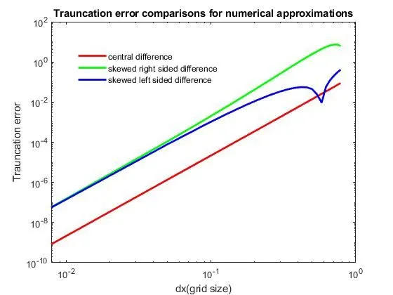
• Then I have plotted the graph dx as x-axis and truncation error as y-axis. Using loglog plot.
• Then I have added labels titles and legends to the plot.

OUTPUT PLOT

CONCLUSION

• From the above plot, we can observe that the order of truncation error is almost same for both skewed right and left difference. for a given grid size(dx), truncation error of central difference is lesser compared to both skewed left and right sided scheme therefore central differencing scheme is comparatively better numerical approximation.
• Since, the central difference numerical scheme takes information from both right and left grid points. Central difference scheme cannot be calculated or may not provide appropriate solution in some flow region such as boundary, shock wave, Central difference fails in boundary regions because it requires information from points beneath the boundary which is out of the computational domain. In such cases, skewed scheme may be preferred.