Week 7 - Auto ignition using Cantera
AUTO IGNITION USING CANTERA
OBJECTIVE:
The main aim of this challenge is to create a reactor network using cantera and capture the Auto Ignition delay for methane combustion under different operating conditions.
Part - I:
- Plot the variation of Auto Ignition time of Methane with a constant temperature of 1250K and pressure varying from 1 to 5 atm.
- Plot the variation of Auto Ignition time of Methane with a constant pressure of 5 atm and temperature varying from 950K to 1450K.
Part - II:
Observe and print the rate of change of molar concentrations of the given elements "H2O, O2, OH" with respect to the time.
- When Temperature is 1000K and pressure 5 bar
- When Temperature is 500K and pressure 5 bar
THEORY:
In simple words, Auto Ignition is defined as the coombustion takes place spontaneously without any external sources when the mixture of the gases reaches certain temperature. The delay which takes before auto ignition is the Auto ignition delay. The Auto Ignition temperature is not an intrensic property of the gases as it is the lowest temperature requried to start the combustion. It is affected by the conditions like pressure, temperature and the composition of the gases.
As at low pressure, the auto ignition temperature will gets increase which increases ignition delay. Similarly at high temperature also, the ignition will take spontaneously. If the compostion is too lean or too rich, it will effect the auto ignition temperature accordingly. All these cases will study in this challenge using Cantera by creating a reactor network.
Part - I:
The first part of this challenge is to create a reactor network using Cantera module by writing code in python. The gas object taking here is the methane and the reactor is considering as Ideal gas reactor by advancing the reactor with 1e-3 s time step for about 1000 steps.
a) Plot the variation of Auto Ignition time of Methane with a constant temperature of 1250K and pressure varying from 1 to 5 atm:
import sys
import cantera as ct
import numpy as np
import matplotlib.pyplot as plt

#Creating a gas object
gas = ct.Solution('gri30.xml')
P_start = 1*101325			#Initial pressure, pa
P_end = 5*101325			#Final pressure
T = 1250   					#Constant temperature, k
Pressure = np.linspace(P_start,P_end,5)
#Creating an array for Ignition delay
Ignition_delay = []

#
for P in Pressure:
	# Setting the Values for the gas object.
	gas.TPX = T,P,{'CH4':1,'O2':2,'N2':7.52}
	r = ct.IdealGasReactor(gas)					#Creating an Ideal gas reactor
	sim = ct.ReactorNet([r]) 					#Creating the sinulation object
	time = 0.0									#Initial time
	T_old = T
	states = ct.SolutionArray(gas,extra = ['time_in_ms','t']) #Creating the states object which sets an array for all propeties of gas at different steps
	#Given simulation time is 10s
	for i in range(10000):
		time += 1e-3			#For every 1e-3s, the solution gets caluculated
		sim.advance(time)		#Integrating the system for given time
		states.append(r.thermo.state, time_in_ms = time*1e-3, t =time)		#Appending all the state values
		T_new = states.T
		T_new = T_new[i-1]

		#Creating an IF loop to caluculate the Ignition delay.
		if T_new>= T_old+400:
			Ignition_delay.append(time)
			T_old = states.T
			T_old = T_old[i-1]

	#PLotting ignition delay at different initial pressures
	plt.figure(1)
	plt.plot(states.time_in_ms, states.T)


print('Ignition Delay = ', Ignition_delay)
print('Pressure =', Pressure)

plt.xlabel('Time [ms]')
plt.ylabel('Temperature [K]')
plt.legend(['P_start =' + str(P) + '[K]' for P in Pressure])
#
plt.figure(2)
plt.plot(Pressure,Ignition_delay,'-o')
plt.xlabel('Pressure [Pa]')
plt.ylabel('Ignition Delay [ms]')
plt.show()
PROCEDURE:
- Importing all the necessary libraries to python.
- Creating a gas object by using solution class of GRI30.xml.
- Creating a for loop with a range of pressure array.
- Setting up the conditions by using gas.TPX method.
- Creating a IdealGasReactor with a object name of r and creating a simulation object.
- Creating the states object which is an array to store all properties at every time step.
- Using time loop and sim.advance method initializing the simulation by integrating at every 1e-3s.
- Appending all the states.
- Creating the if loop to caluculate the Ignition delay.
- Plotting the results.
PLOTS:
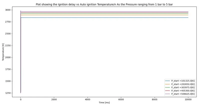
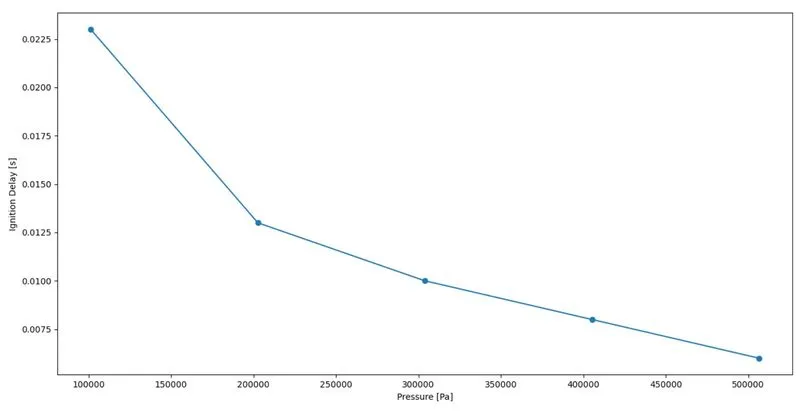
| Temperature, k | Ignition delay |
| 950 | 0.427 |
| 1075 | 0.055 |
| 1200 | 0.011 |
| 1325 | 0.004 |
| 1450 | 0.001 |
OBSERVATION:
From the above plots , we can understand that the ignition delay is decreasing with the increase in Initial temperature. So that the ignition delay is dependant on the initial temperature of the fuel.
b) Plot the variation of Auto Ignition time of Methane with a constant pressure of 5 bar and temperature varying from 950k to 1450k:
import sys
import cantera as ct
import numpy as np
import matplotlib.pyplot as plt

#Creating a gas object
gas = ct.Solution('gri30.xml')
T_start = 950
T_end = 1450
Temperature = np.linspace(T_start,T_end,5)   #k
P = 5*101325    #N/m^2
Ignition_delay = []

for T in Temperature:

	gas.TPX = T,P,{'CH4':1,'O2':2,'N2':7.52}
	r = ct.IdealGasReactor(gas)				#Creating an Ideal gas reactor
	sim = ct.ReactorNet([r])				#Creating the sinulation object
	time = 0.0								#Initial time
	T_old = T
	states = ct.SolutionArray(gas,extra = ['time_in_ms','t'])	#Creating the states object which sets an array for all propeties of gas at different steps
	#i = 1
	for i in range(10000):
		time += 1e-3		#For every 1e-3s, the solution gets caluculated
		sim.advance(time)	#Integrating the system for given time
		states.append(r.thermo.state, time_in_ms = time*1e3, t =time)	#Appending all the state values
		T_new = states.T
		T_new = T_new[i-1]

		if T_new>= T_old+400:
			Ignition_delay.append(time)
			T_old = states.T
			T_old = T_old[i-1]

	#Plotting the Ignition delay vs auto ignition temperature at different initial temperatures
	plt.figure(1)
	plt.plot(states.time_in_ms, states.T)


print('Ignition Delay = ', Ignition_delay)
print('Temperature =', Temperature)


plt.xlabel('Time [ms]')
plt.ylabel('Temperature [K]')
plt.legend(['T_start =' + str(T) + '[K]' for T in Temperature])
plt.title('Plot showing the Ignition delay as the Initial temperatures ranging from 950k to 1450k')

# Plotting Temperature vs Ignition delay
plt.figure(2)
plt.plot(Temperature,Ignition_delay,'-o')
plt.xlabel('Temperature [k]')
plt.ylabel('Ignition Delay [s]')
plt.show()
PROCEDURE:
- Importing all the necessary libraries to python.
- Creating a gas object by using solution class of GRI30.xml.
- Creating a for loop with a range of temperature array.
- Setting up the conditions by using gas.TPX method.
- Creating a IdealGasReactor with a object name of r and creating a simulation object.
- Creating the states object which is an array to store all properties at every time step.
- Using time loop and sim.advance method initializing the simulation by integrating at every 1e-3s.
- Appending all the states.
- Creating the if loop to caluculate the Ignition delay.
- Plotting the results.
RESULTS:
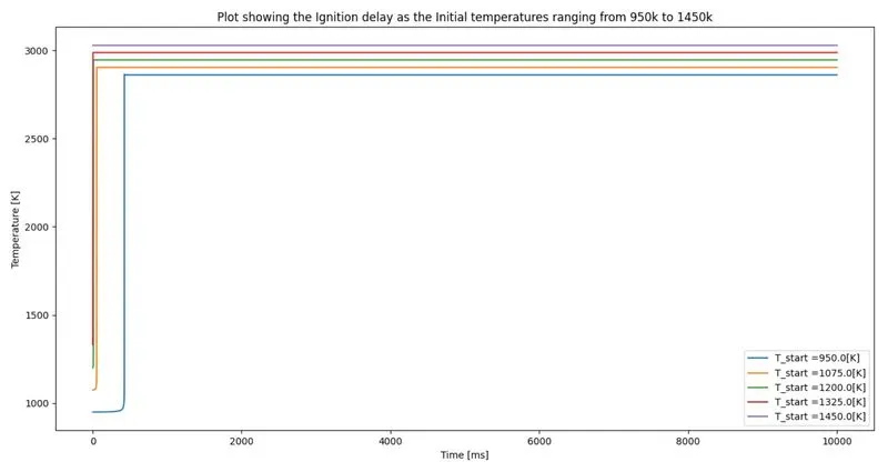
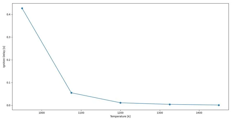
| Initial Pressure, Pa | Ignition Delay |
| 101325 | 0.023 |
| 202650 | 0.013 |
| 303975 | 0.010 |
| 405300 | 0.008 |
| 506625 | 0.006 |
OBSERVATION:
The above plot is very similar to the temperature varying plot as the ignition delay is increasing with the decrease in the initial pressure. One more thing need to observe from first plot is that the decreased pressure incraesing the auto ignition temperature, so that the ignition delay is sensitive to Initial pressure.
PART - II:
Observe and print the rate of change of molar concentrations of the given elements "H2O, O2, OH" with respect to the time.
import sys
import cantera as ct
import numpy as np
import matplotlib.pyplot as plt

#Creating a gas object
gas = ct.Solution('gri30.xml')
T_start = 950
T_end = 1450
Temperature = [500,1000]   #k
P = 5*101325    #N/m^2
Ignition_delay = []

for T in Temperature:

	gas.TPX = T,P,{'CH4':1,'O2':2,'N2':7.52}
	r = ct.IdealGasReactor(gas)				#Creating an Ideal gas reactor
	sim = ct.ReactorNet([r])				#Creating the sinulation object
	time = 0.0								#Initial time
	T_old = T
	states = ct.SolutionArray(gas,extra = ['time_in_ms','t'])	#Creating the states object which sets an array for all propeties of gas at different steps
	#i = 1
	for i in range(1000):
		time += 1e-3			#For every 1e-3s, the solution gets caluculated
		sim.advance(time)		#Integrating the system for given time
		states.append(r.thermo.state, time_in_ms = time*1e3, t =time)	#Appending all the state values


	#PLotting the ignition delay vs Species Concentration of H2O
	plt.figure(1)
	plt.plot(states.t,states.X[:,gas.species_index('H2O')])
	plt.xlabel('Time [s]')
	plt.ylabel('Species Concentration [H2O]')
	#PLotting the ignition delay vs Species Concentration of O2
	plt.figure(2)
	plt.plot(states.t,states.X[:,gas.species_index('O2')])
	plt.xlabel('Time [s]')
	plt.ylabel('Speies Concentration O2')
	#PLotting the ignition delay vs Species Concentration of OH
	plt.figure(3)
	plt.plot(states.t,states.X[:,gas.species_index('OH')])
	plt.xlabel('Time [s]')
	plt.ylabel('Species Concentration [OH]')
	plt.show()
PROCEDURE:
- Importing all the necessary libraries to python.
- Creating a gas object by using solution class of GRI30.xml.
- Creating a for loop with a range of temperature array and a constant pressure of 5 bars for both cases.
- Setting up the conditions by using gas.TPX method.
- Creating a IdealGasReactor with a object name of r and creating a simulation object.
- Creating the states object which is an array to store all properties at every time step.
- Using time loop and sim.advance method initializing the simulation by integrating at every 1e-3s.
- Appending all the states.
- Plotting the results by using states.X[:,gas.species_index('species')] vs staes.t
RESULTS:
When Temperature is 500K and pressure 5 bar:
OBSERVATION:
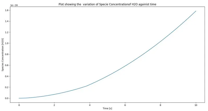
- From the plot of species concentration of H2O, we can observe that at initial stage the concentration is at nothing as the combustion is going on the comcentration is increasing with the time. The plot makes sense as we know H2O species will form as products of methane combustion, so initially with zero concentration will goes on increasing as the combustion time increasing.
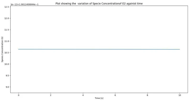
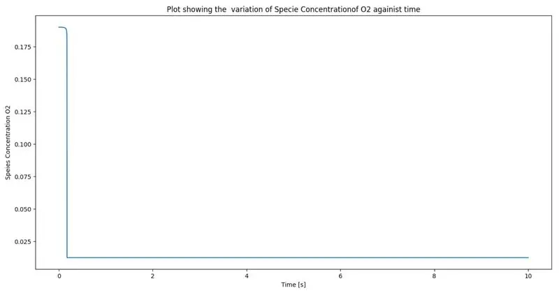
- From the second plot, we can observe that the oxygen concentration is at constant rate, although the time increasing. This is because the initial temperature, we set here is 500k, so untill reaching the auto ignition temperature we need to supply the oxygen to start the combustion.
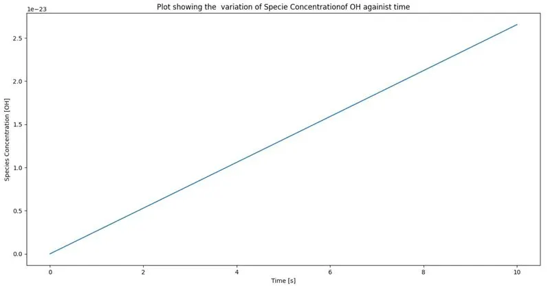
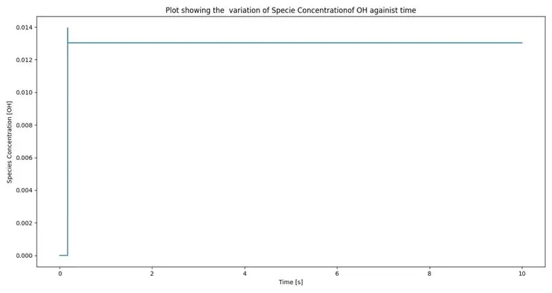
- From the third plot, the concentration of OH is at zero, as the time increasing it keeps increasing proportrionally. This also makes sense that as the initial temperature is minimal, untill reaching the Auto Ignition temperature, the elementary reaction of OH will keep gets inceasing with time being.
When Temperature is 500K and pressure 5 bar:
OBSERVATION:
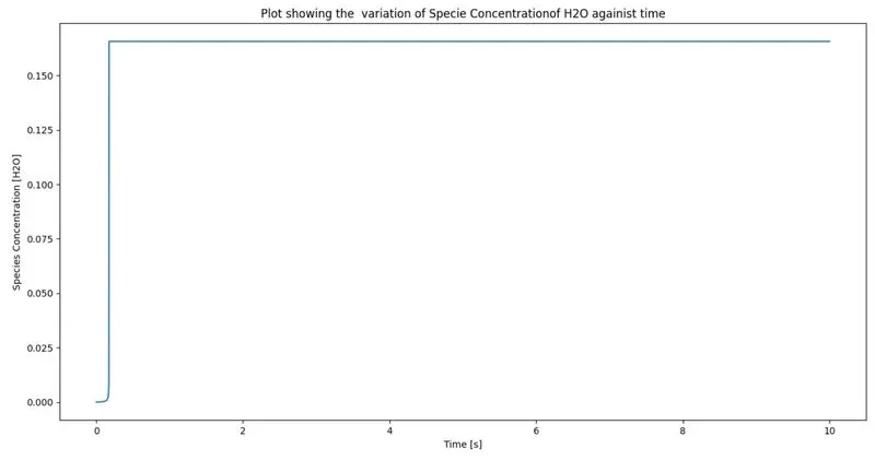
- From the first plot, we can observe a variation from case - I, as the concentration of the H2O is zero initially but with the incraese in the time, there is a rise in the concentration at certain time and after reaching maximum concentration, it keeps at constant. This makes sense as the initial temperature considering here is 1000k, which is auto iginition temperature, so the iginition takes within no time and the formation of H2O gets increased after complete combustion, it gets at constant concentraction as the mixture we are considered is stoichometric.
- From the second plot, we can observe that after reaching Auto ignition temperature, the concentration of oxygen is getting decreased and gets to constant after some time. This is beacause, after having enough concentration to combust methane, the combustion will takes place.
- From the third plot comparing with case-I, we can observe the difference in the concentration of OH. As in the first case, it is upto 2.8 percent, but in second case it is of 0.013. This is because as the initial temperature is enough to Auto ignite, the number of elementary reaction will gets reduced to complete the combustion, as the mixture is stoichometric, the concentration of OH will be very minimal which makes sense.
CONCLUSION:
By simulating the above cases, we can conclude that the Auto ignition delay is sensitive to Initial temperature, pressure an the species concentration(mostly depends of the concentration of O2). Increase or decrease any of above three will makes impact of ignition delay and Auto ignition temperature.