Week 6: Shock tube simulation project

Shock Tube Simulation

• Aim:

To perform a Shock tube simulation using the transient state approach. Using an event method in intial conditions to set a time to break the diaphragm and the mixing of high pressure region and low pressure region to occur. Post process the results and explain the flow physics.

• Theory:

1. Shock Tube:

The shock tube is an instrument used to replicate and direct blast waves at a sensor or a model in order to simulate actual explosions and their effects, usually on a smaller scale. Shock tubes (and related impulse facilities such as shock tunnels, expansion tubes, and expansion tunnels) can also be used to study aerodynamic flow under a wide range of temperatures and pressures that are difficult to obtain in other types of testing facilities. Shock tubes are also used to investigate compressible flow phenomena and gas phase combustion reactions. More recently, shock tubes have been used in biomedical research to study how biological specimens are affected by blast waves.

2. Regions and Events:

In Converge, a 'Region' is a collection of boundaries used to delineate different areas in a geometry. Let us take the example of the shock tube itself. In the shock tube, there exists a High-pressure(HP) region and a Low-pressure(LP) region. These two must be separated initially which is taken care of by regions.

Events is a feature that engages and disengages two boundaries. In a real shock tube, there is a diaphragm that prevents mixing between the two chambers. To incorporate this effect in the simulation, a region is added, and using events, the disengagement of the region is simulated. At time t>0, the initial engagement is disengaged and the pressure difference creates a shockwave.

Internally, the Converge solver creates a temporary obstruction using triangles to from regions. These temporary triangles are called Disconnect Triangles. There are two types of disconnect triangles- Single Loop and Concentric.

In the shocktube simulation, single-loop disconnect triangles are used, as the interface region between both the regions are of the same dimensions

• Procedure:

1. Load the STL file and flag the boundary regions accordingly assigning the high-pressure and low pressure regions in the geometry.

2. Remove the coinciding wall inbetween the high and low pressure region walls so that non-manifold errors can be avoided.

3. Transform the normal inside the fluid flow regions.

- Case setup:

1. Application type: time based

2. Materials:

a. Gas simulation: air

b. Solid simulation: Aluminium

c. Global transport properties: Deafult

d. Species:

gases: O2 and N2

3. Simulation parameters:

a. Run parameters:

Transient solver, full hydrodynamic, compressible

b. Simulation time parameters:

- End time- 0.003 sec

- Time step- 1e-09

- min time step- 1e-09

- max time step- 1

- Convection CFL number- 0.5

c. Solver Parameters-

- Solver type- density based solver

4. Boundary Conditions-

a. High pressure region:

- Temperature BC- Nueman BC

- Velocity BC: Stationary, Slip

b. Low pressure region:

- Temperature BC- Nueman BC

- Velocity BC: Stationary, Slip

5. Initial Conditions and Events:-

- Regions and Initialization:

1. High pressure region:

Temperature: 300K

Pressure: 6 Bar

Species: N2 (mass fraction: 1)

2. Low pressure region:

Temperature: 300K

Pressure: 1 Bar

Species: O2 (mass fraction: 1)

- Events:

Sequential:

Start - 0 sec, region A: High Pressure, region B: Low pressure, event: CLOSE

Break diaphargm- 0.001sec, region A: High Pressure, region B: Low pressure, event: OPEN

6. Physical Models:-

- RNG k-epsilon

7. Grid Control:-

a. Base Grid:

dx = 1e-4m, dy = 1e-4m, dz = 1e-4m

b. Addaptive mesh refinement:

Min and Max cells: 0, 200000

Species refinement type-

name: N2, timing type: Permanent, GS embedding scale: 0.001, embedded scale: 3

8. Post-Processing:-

- Post Variable Selection:

Select the parameters needed to be post processed.

- Output files:

We need to set a time interval for the files to be saved during each set of iterations. It is best suited to have a min of 100 saved files for every simulation. Therefore we need to calculate the time interval for writing the output files based on our end time given in run parameters.

Restart files help in restoring the files if there is a sudden power cut/ crash which is not helpful or might end up loosing the entire data, therefore the restart files helps in resuming the simulation form the point we lost contact. Restart files time interval can be same as the writing files interval which is safe and healthy.

In this case- since the end time is 0.003, we can have a time interval of 1e-05 and the total files created will be 100.

• Results:

1. Mesh:

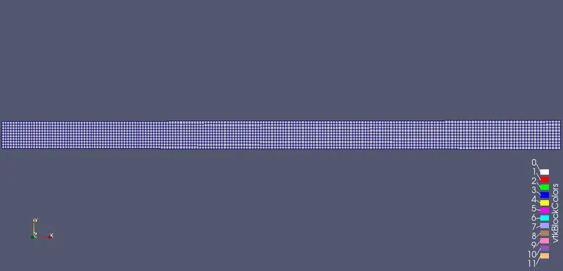
- Mesh grid:

- Cell count:

- AMR animation:

- Discussions:

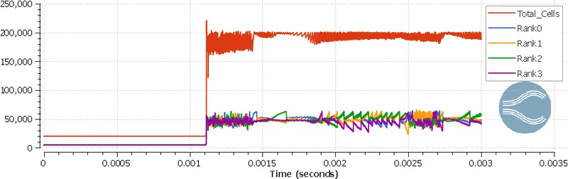
The total cell count plot shows the variation of mesh sizes as a function of time during the entire simulation of 0.003 seconds. In the events option setting has done for the diaphragm to burst at 0.001 seconds as a result of that diaphragm bursting sudden spike is observed after 0.001 seconds i.e interaction of two regions. When the simulation begins the high-pressure region pushes the low-pressure region and the AMR gets activated, the variations of which can be observed in the plot. The sudden decrease in mesh size is when the reflected pressure pushes it back.

2. Pressure regions contour:

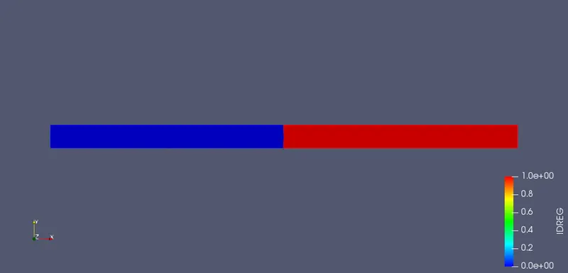
Blue being the High Presure region and Red being the Low pressure region, Have used the Blue to red Colour map.

3. Temperature:

- Temperature plot:

- Temperature contour:

- Temperature animation:

4. Pressure:

- Pressure plot:

- Pressure contour:

- Pressure aimation:

5. Velocity:

- Velocity contour:

- Velocity animation:

• Discussions:

- Temperature:

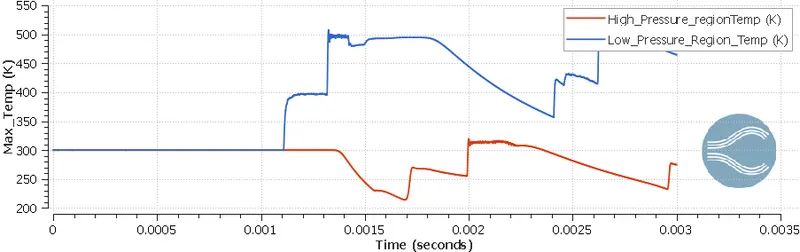
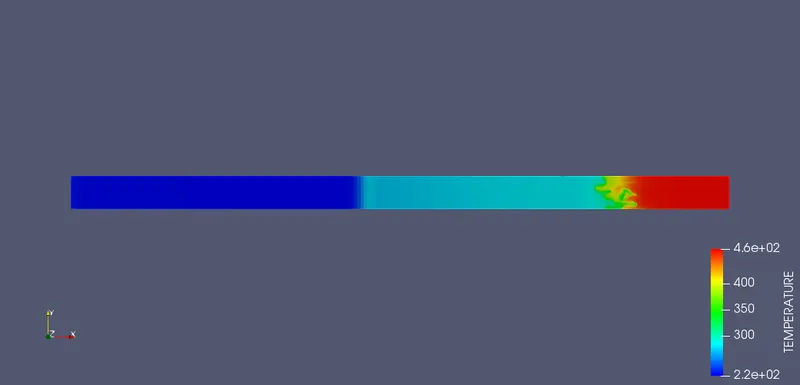
• The temperature is initially 300K at both the regions. Once the diaphragm breaks, due the pressure difference, the shockwaves sets in and this causes an increase in temperature in the driven region.
• Towards the left side of the diaphragm (driver region), rarefaction waves are set into motion, which casuses the expansion process, and hence there is a decrease in temperature from the ambient.
• When the shockwave hits the right end, its temperature increases further and gets reflected back. It now travels towards the other end of the tube heating the contents of the tube even at the driver side where the contents are below ambient temperature due to the rarefaction wave.
• Upon getting reflected back, its temperature further increases, and once again it travels towards the right end heating all the contents as it propagates.
• When it hits the right end the second time, the temperature reaches a local maxium and this process keeps repeating.

- Pressure:

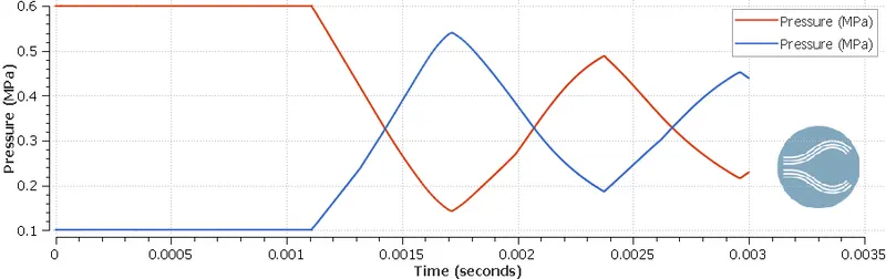
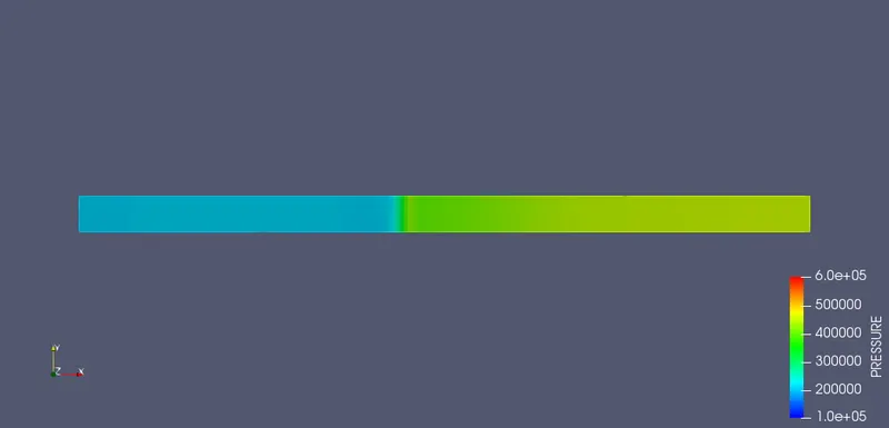
The High-pressure region is at 6 Bar and from the plot, it is clearly visible that simulation never reaches that pressure. As soon as the diaphragm breaks at 0.001 seconds the pressure increases and the high-pressure region pushes the low-pressure region again low-pressure region pushes high-pressure region and it is just like pushing and dissolving until reflected wave can occur. Generation of a shock wave in the low-pressure region leads to pressure rise and a slight drop in the plot is visible.

Both the regions generate a sine wave-like structure with their shock waves. This pressure eventually dissolves into steady value when a simulation is run for more time steps.

• Conclusion:

The shock tube is mainly used to study the properties of the fluid at an elevated temperature and pressure.

The burst of the diaphragm creates compression waves which propagate in the driven section and expansion waves traversing in the driver section.

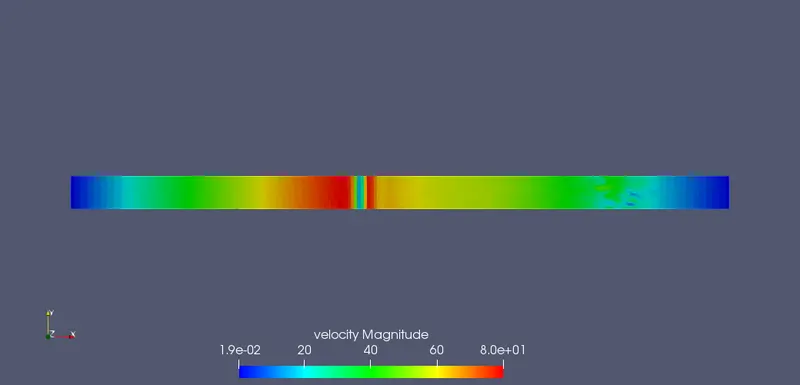
The shock wave when hits the wall gets refracted back and the mixing of the fluid occurs. The pressure gradients between driver and driven section are due to viscous drag and friction between shock wavefront and shock tube walls.

The gas behind the reflected wave is at rest relative to the shock tube. Usually, there is some mixing and interdiffusion of gases at the contact surface so that the temperature fall is less sudden than in the ideal case. In the case of IC engines, this shock tube data is important to find the ignition delay i.e, how long it takes to ignite fuel and air