Week 6 - Multivariate Newton Rhapson Solver

Assignment number 06

Title-Multivariate Newton Raphson technique

Aim- to solve the set of ODE equations using multivariate Newton Raphson Technique.

The given set of ODE’s are

dy1/dt= -0.04*y1+〖10〗^4*y2*y3  
dy2/dt= 0.04*y1-〖10〗^4*y2*y3-3*〖10〗^7*〖y2〗^2  
dy3/dt=3*〖10〗^7*〖y2〗^2  

The problem is discretised using Implicit Euler Method/Backward Differencing.

(〖y1〗^n-〖y1〗^(n-1))/∆t=-0.04*y1+〖10〗^4*y2*y3  
(〖y2〗^n-〖y2〗^(n-1))/∆t=0.04*y1-〖10〗^4*y2*y3-3*〖10〗^7*〖y2〗^2
(〖y3〗^n-〖y3〗^(n-1))/∆t=3*〖10〗^7*〖y2〗^2

Rearrange the above equation in terms of RHS-LHS=0 we get following non linear equation

f1=〖y1〗^(n-1)+∆t*(-0.04*y1+〖10〗^4*y2*y3)-〖y1〗^n
f2=〖y2〗^(n-1)+∆t*( 0.04*y1-〖10〗^4*y2*y3-3*〖10〗^7*〖y2〗^2 )-〖y2〗^n
f3=〖y3〗^(n-1)+∆t*(3*〖10〗^7*〖y2〗^2 )-〖y3〗^n

Where,

y^n=value at current time steps
y^(n-1)=value at previous time steps

The newton Raphson formula is given as

Y_new=Y_guess-∝*J^(-1)*F

The initial values taken as

〖Y1〗_guess=1
〖Y2〗_guess=0
〖Y3〗_guess=0

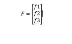
Matrix F is the column matrix of the functions,

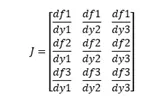
Jacobian matrix is given as

∝=1

Coding approach

• First simply of all ODE’s
• Then define function for each ODE’s
• Also define function for jacobian matrix
• Outer time integration loop
• Assembling ODE’s and newton Raphson till we get results
• End time loop
• Insert your graphs in report

Note-simulation is run for 10 minute i.e. 600s

Code

"""
multivaiate newton rhapson technique

date-26-1-2022

author = siddhesh sakpal

"""
import numpy as np
import matplotlib.pyplot as plt
from numpy.linalg import inv

 #define function for each ode

def f1(y1_old,y1,y2,y3,dt):
 	return y1_old + dt*(-0.04*y1 + 1e4*y2*y3)-y1

def f2(y2_old,y1,y2,y3,dt):
 	return y2_old + dt*(0.04*y1 - 1e4*y2*y3-3e7*y2**2)-y2
 
def f3(y3_old,y1,y2,y3,dt):
 	return y3_old + dt*(3e7*y2**2)-y3

def jacobian(y1_old,y2_old,y3_old,y1,y2,y3,dt):

	J=np.ones((3,3))
	h=1e-7

	#ROW 1
	J[0,0]=(f1(y1_old,y1+h,y2,y3,dt)-f1(y1_old,y1,y2,y3,dt))/h
	J[0,1]=(f1(y1_old,y1,y2+h,y3,dt)-f1(y1_old,y1,y2,y3,dt))/h
	J[0,2]=(f1(y1_old,y1,y2,y3+h,dt)-f1(y1_old,y1,y2,y3,dt))/h

	#ROW2
	J[1,0]=(f2(y2_old,y1+h,y2,y3,dt)-f2(y2_old,y1,y2,y3,dt))/h
	J[1,1]=(f2(y2_old,y1,y2+h,y3,dt)-f2(y2_old,y1,y2,y3,dt))/h
	J[1,2]=(f2(y2_old,y1,y2,y3+h,dt)-f2(y2_old,y1,y2,y3,dt))/h

	#ROW3
	J[2,0]=(f3(y3_old,y1+h,y2,y3,dt)-f3(y3_old,y1,y2,y3,dt))/h
	J[2,1]=(f3(y3_old,y1,y2+h,y3,dt)-f3(y3_old,y1,y2,y3,dt))/h
	J[2,2]=(f3(y3_old,y1,y2,y3+h,dt)-f3(y3_old,y1,y2,y3,dt))/h

	return J

# initial condition
y1=1
y2=0
y3=0

 #guess
y_guess=np.ones((3,1))
y_guess[0]=y1
y_guess[1]=y2
y_guess[2]=y3

y_old=np.ones((3,1))
y_old[0]=y1
y_old[1]=y2
y_old[2]=y3

F=np.copy(y_guess)
alpha=1
tol=1e-6
dt=20
#final values
y_new1=[]
y_new2=[]
y_new3=[]
time=np.arange(0,600,dt) 
iter=1

for t in np.arange(0,600,dt):
	error=9e9
	while error>tol:
		J=jacobian(y_old[0],y_old[1],y_old[2],y_guess[0],y_guess[1],y_guess[2],dt)
		F[0]=f1(y_old[0],y_guess[0],y_guess[1],y_guess[2],dt)
		F[1]=f2(y_old[1],y_guess[0],y_guess[1],y_guess[2],dt)
		F[2]=f3(y_old[2],y_guess[0],y_guess[1],y_guess[2],dt)

		ynew=y_guess-alpha*np.matmul(inv(J),F)

		error=np.max(np.abs(ynew-y_guess))

		y_guess=ynew

		iter=iter+1

		log_message='iteration  #={0} y1={1} y2={2} y3={3}' . format(iter,ynew[0],ynew[1],ynew[2])

		print(log_message)
	y_old=ynew
	y_new1.append(ynew[0])
	y_new2.append(ynew[1])
	y_new3.append(ynew[2])

plt.plot(time,y_new1,label='y1')
plt.plot(time,y_new2,label='y2')
plt.plot(time,y_new3,label='y3')
plt.xlabel=('time in sec')
plt.ylabel('Y')
plt.legend()
plt.grid()
plt.show()

graphs

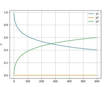
dt= 0.5s

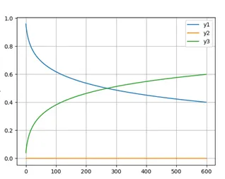
dt=1.5s

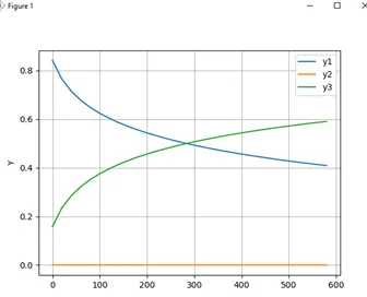
dt=20s

Results and conclusion

• From the above graphs if we decrease the time step, the number of iteration increases hence obviously increases computational time. There is not much difference but with larger time steps the accuracy has been compromised
• When the time steps are varied the solution is stable throughout and there is no any changes in solution that why we used implicit method and it is not possible with explicit method