Week 6 - Multivariate Newton Rhapson Solver

STUDY ON MULTIVARIATE
NEWTON RAPHSON SOLVER

Aim:

To solve the given set of equations using Multivariate Newton Rhapson technique for suitable timestep and by estimating the Jacobian numerically.

Equations:

`dy_1/dt = -0.04y_1 + 10^4y_2y_3`
`dy_2/dt = 0.04y_1 - 10^4y_2y_3 - 3*10^7y_2^2`
`dy_3/dt = 3*10^7y_2^2`

Theory:

Newton Raphson Method:

In numerical analysis, Newton's method, also known as the Newton–Raphson method, is a root-finding algorithm which produces successively better approximations to the roots (or zeroes) of a real-valued function. The idea is to start with an initial guess which is reasonably close to the true root, then to approximate the function by its tangent line using calculus, and finally to compute the x-intercept of this tangent line by elementary algebra. This x-intercept will typically be a better approximation to the original function's root than the first guess, and the method can be iterated.

So, based on the number of iterations, the solution will be converging to a better and more accurate finding with minimal error. It's equation is as follows;

`Y_(n+1) = Y_n - alpha.J^-1F(Y)`
where, `Y_(n+1)` is the matrix for new values for `y_(1,2,3,..,n)`
`Y_(n)` is the matrix for old or previous values for `y_(1,2,3,..,n)`, initially it is guess values
`alpha` is the relaxation factor
`F(Y)` is the function which has the equations of `Y` to determine each root values and
`J` is the Jacobian matrix which contains all possible derivatives of `Y` w.r.t `F`

Procedure:

⦁ To solve the given set of equations, we use Python programming language for simplicity in handling large number of iterations.

"""
Program to study Multivariate Newton Rhapson Solver:

Equations;

dy1/dt = -0.04*y1 + pow(10,4)*y2*y3
dy2/dt = 0.04*y1 - pow(10,4)*y2*y3 - 3*pow(10,7)*y2*y2
dy3/dt = 3*pow(10,7)*y2*y2
"""
import numpy as np 
from numpy.linalg import inv
import matplotlib.pyplot as plt 

# Time Interval
t_start = 0
t_end = 600 # Simulation for 10 mins = 600 s
n = 6000 # Number of timesteps
dt = (t_end - t_start)/n # Size of each timestep

Iter = 0

# Initial Guess Value
y1 = 1
y2 = 0
y3 = 0

# Function definition;

def f1(y1_old,y2_old,y3_old,y1,y2,y3,dt):
	
	# First Non - Linear Equation

	return y1_old + (-0.04*y1 + pow(10,4)*y2*y3)*dt - y1

def f2(y1_old,y2_old,y3_old,y1,y2,y3,dt):
	 
	# Second Non - Linear Equation

	return y2_old + (0.04*y1 - pow(10,4)*y2*y3 - 3*pow(10,7)*y2*y2)*dt - y2

def f3(y1_old,y2_old,y3_old,y1,y2,y3,dt):
	
	# Third Non - Linear Equation

	return y3_old + (3*pow(10,7)*y2*y2)*dt - y3

# Jacobian Matrix using Numerical computation method;

def jacobian(y1_old,y2_old,y3_old,y1,y2,y3,dt):
	
	J = np.zeros((3,3)) # Initialization of the Jacobian matrix
	h = 1e-4 # A very small increment for the variable values to compute the Jacobian numerically

	# First Row
	J[0,0] = (f1(y1_old,y2_old,y3_old,y1+h,y2,y3,dt)-f1(y1_old,y2_old,y3_old,y1,y2,y3,dt))/h
	J[0,1] = (f1(y1_old,y2_old,y3_old,y1,y2+h,y3,dt)-f1(y1_old,y2_old,y3_old,y1,y2,y3,dt))/h
	J[0,2] = (f1(y1_old,y2_old,y3_old,y1,y2,y3+h,dt)-f1(y1_old,y2_old,y3_old,y1,y2,y3,dt))/h

	# Second Row 
	J[1,0] = (f2(y1_old,y2_old,y3_old,y1+h,y2,y3,dt)-f2(y1_old,y2_old,y3_old,y1,y2,y3,dt))/h
	J[1,1] = (f2(y1_old,y2_old,y3_old,y1,y2+h,y3,dt)-f2(y1_old,y2_old,y3_old,y1,y2,y3,dt))/h
	J[1,2] = (f2(y1_old,y2_old,y3_old,y1,y2,y3+h,dt)-f2(y1_old,y2_old,y3_old,y1,y2,y3,dt))/h

	# Third Row
	J[2,0] = (f3(y1_old,y2_old,y3_old,y1+h,y2,y3,dt)-f3(y1_old,y2_old,y3_old,y1,y2,y3,dt))/h
	J[2,1] = (f3(y1_old,y2_old,y3_old,y1,y2+h,y3,dt)-f3(y1_old,y2_old,y3_old,y1,y2,y3,dt))/h
	J[2,2] = (f3(y1_old,y2_old,y3_old,y1,y2,y3+h,dt)-f3(y1_old,y2_old,y3_old,y1,y2,y3,dt))/h

	return J



# Newton Rhapson Method

def Solver_N(y1,y2,y3,y1_guess,y2_guess,y3_guess,dt):
	
	global Iter
	Y_old = np.zeros((3,1)) # Initializing and populating Y_old with the guess values
	Y_old[0] = y1_guess
	Y_old[1] = y2_guess
	Y_old[2] = y3_guess

	F = np.zeros((3,1)) # Initializing the function vector

	error = 9e9 # Error criteria
	tol = 1e-4 # Tolerance value
	alpha = 1 # Relaxation factor

	while(error>tol): # Inner loop for satisfying the error tolerance for a given time step;
		
		# Calling the Jacobian function, with Initial and Guess values for y;
		J = jacobian(y1,y2,y3,Y_old[0],Y_old[1],Y_old[2],dt)

		F[0] = f1(y1,y2,y3,Y_old[0],Y_old[1],Y_old[2],dt)
		F[1] = f2(y1,y2,y3,Y_old[0],Y_old[1],Y_old[2],dt)
		F[2] = f3(y1,y2,y3,Y_old[0],Y_old[1],Y_old[2],dt)

		Y_new = Y_old - alpha*(np.matmul(inv(J),F))
		error = np.max(np.abs(Y_new-Y_old))
		
		Y_old = Y_new # Setting the new values of y to y_old, to continue iteration until error < tol
		
		log_message = 'Iteration = {0}, y1 = {1}, y2 = {2}, y3 = {3}'.format(Iter,Y_new[0],Y_new[1],Y_new[2])
		print(log_message)
		
		Iter = Iter + 1

	return [Y_new[0],Y_new[1],Y_new[2]]

# Implicit Euler

t = np.arange(t_start,t_end,dt)

Y_1 = np.zeros(len(t))
Y_2 = np.zeros(len(t))
Y_3 = np.zeros(len(t))

Y_1[0] = y1
Y_2[0] = y2
Y_3[0] = y3

y1_guess = 0
y2_guess = 0
y3_guess = 0

for i in range (1,len(t)):
	
	# For each and every New value of y, we capture the Y_1, Y_2 & Y_3 values for every timestep;
	Y_1[i],Y_2[i],Y_3[i] = Solver_N(Y_1[i-1],Y_2[i-1],Y_3[i-1],y1_guess,y2_guess,y3_guess,dt)

	# Re-initializing guess values with the new values for y respectively, for every timestep;
	y1_guess = Y_1[i] 
	y2_guess = Y_2[i]
	y3_guess = Y_3[i]

# Plotting the graph for Values of y1, y2 & y3 in every time steps;

plt.plot(t,Y_1,'-')
plt.plot(t,Y_2,'--')
plt.plot(t,Y_3,'-.')
plt.xlabel('Simulation Time (s)')
plt.ylabel('Variables (units)')
plt.legend(['y1','y2','y3'])
plt.title('Multivariate Newton Rhapson Solver, dt = 0.1')
plt.grid('on')
plt.show()

⦁ For this program, we define 4 different in-stream functions, namely f1, f2, f3, jacobian and Solver_N which are self explanatory. the functions f1, f2 and f3 contains the derivative equations of y1, y2 and y3 with respect to t. The Jacobian function is used to define the Jacobian Matrix which consists of all possible derivatives which is solved numerically by applying Explicit interpolation technique.
⦁ Now, the last function is the solver which consists of the Newton Raphson equation for non-linear functions. This is where all the values of variables in a given time step is calculated. So for each and every time step, the New values for Y_new is calculated and plotted as a function of 't'.

Results:

Thus, the given set of equations using Multivariate Newton Rhapson technique for suitable timestep and by estimating the Jacobian numerically are solved successfully.

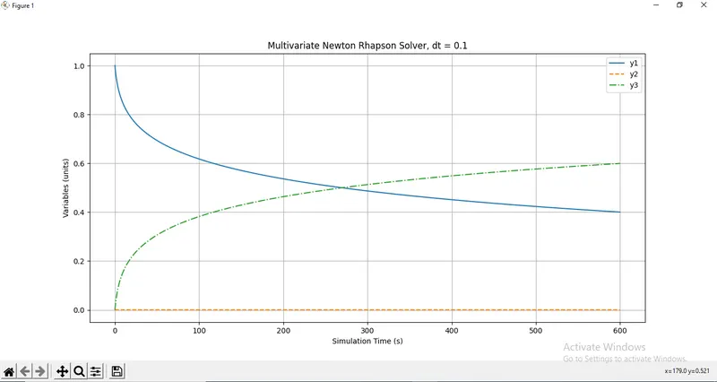
Iteration = 7150, y1 = [0.40047735], y2 = [2.63729471e-06], y3 = [0.59952001]

As we can see, only for explicit method, we can consider the time step as a major criteria as it is directly dependant on it. In our case, we used dt = 0.1 s, since we use an implicit solver like Newton Raphson solver, stability is not majorly affected, but the accuracy of the solution we obtain is majorly affected. For a given time period, if we have a tolerance value for error in the convergence, we might converge to the desired solution quicker if we use a larger time step but we may need to sacrifice the accuracy of results. So, it is upto the user, if he wants a more precise solution, they can go for a very smaller time step which increase the simulation time, but if the user is less focused on the solution accuracy, then he might go for a slightly larger time step within a certain range of acceptable error or deviation. However, if we use an abruptly larger time step, then the solution might diverge or converge with a meaningless solution. As a whole, in our equations, dt = 0.1 (at 7150 iterations), gives an ideal solution with minimal error.