Week 6 - Multivariate Newton Rhapson Solver

Multivariate Newton Rhapson Solver

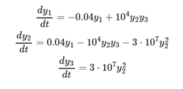
Newton Raphson Method is an iterative technique for solving a set of various nonlinear equations with an equal number of unknowns. There are two methods of solutions for the load flow using the Newton Raphson Method. The first method uses rectangular coordinates for the variables while the second method uses the polar coordinate form. This method is also instrumental in carrying out position analysis of kinematic chains. Following is the system of Non-linear ODE.

--> We have to use an implicit scheme for stable solutions.

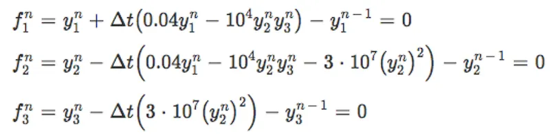
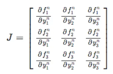
--> This formula is used for the Multi-variable Newton-Raphson technique for solving the coupled equations. J is the Jacobian Matrix which is also described. The update formula also has a relaxation parameter (alpha).

-->Following is the python code for the problem.

import math 
import numpy as np
from numpy.linalg import inv
import matplotlib.pyplot as plt
'''
Multivariate Newton Raphson Method for solving a coupled non-linear 1st order ODE system.
Following is the ODE system
1. We solve the following system of 1st order ODE system using Multivariate N-R Method.
dy1/dt = -0.04*y1 +  y2y3*10e4
dy2/dt = 0.04*y1 +  y2y3*10e4 - 3*(10e7)*y2*y2
dy3/dt = 3*(10^7)*y2*y2
Xnew = Xold - alpha*invJ(F)
'''
iter = 1
# Time loop
dt=0.1 # in seconds
nt=6000 # No. of Time-steps

# Initial Condition
y1_initial=1
y2_initial=0
y3_initial=0

def f1(x1, x2, x3):
		
	return (-0.04*x1 + 10000*x2*x3)*dt - x1 

def f2(x1, x2, x3):
		
	return (0.04*x1 - 10000*x2*x3 - 3*10000000*x2*x2)*dt - x2 

def f3(x1, x2, x3):
		
	return (3*10000000*x2*x2)*dt - x3 

def Jacobian(x1, x2, x3):

	"""
	defining the Jacobian Matrix
	"""
	J = np.ones((3,3))
	# Numerical calculation of the derivatives
	J[0,0]= (f1(x1+1e-8, x2, x3)-f1(x1, x2, x3))/1e-8
	J[0,1]=(f1(x1, x2+1e-8, x3)-f1(x1, x2, x3))/1e-8
	J[0,2]=(f1(x1, x2, x3+1e-8)-f1(x1, x2, x3))/1e-8
	J[1,0]= (f2(x1+1e-8, x2, x3)-f2(x1, x2, x3))/1e-8
	J[1,1]=(f2(x1, x2+1e-8, x3)-f2(x1, x2, x3))/1e-8
	J[1,2]=(f2(x1, x2, x3+1e-8)-f2(x1, x2, x3))/1e-8
	J[2,0]= (f3(x1+1e-8, x2, x3)-f3(x1, x2, x3))/1e-8
	J[2,1]=(f3(x1, x2+1e-8, x3)-f3(x1, x2, x3))/1e-8
	J[2,2]=(f3(x1, x2, x3+1e-8)-f3(x1, x2, x3))/1e-8
	return J

X_old = np.ones((3,1))
X_old[0]=1
X_old[1]=0
X_old[2]=0

F=np.copy(X_old)
error = 9e9

# Parameters for Newton-Raphson Method
Tol=1e-8
alpha=1

# Solution Matrix 
Y_sol = np.ones((3,nt+1))
Y_sol[0,0]=0.99615133
Y_sol[1,0]=3.56511605e-05
Y_sol[2,0]=0.00381302
'''
Y_sol[0,1]=0.99615133
Y_sol[1,1]=3.56511605e-05
Y_sol[2,1]=0.00381302
'''
for i in range(nt):

	while error > Tol:
		J = Jacobian(X_old[0], X_old[1], X_old[2])
		F[0,0]= f1(X_old[0], X_old[1], X_old[2]) + Y_sol[0,i]
		F[1,0]= f2(X_old[0], X_old[1], X_old[2]) + Y_sol[1,i]
		F[2,0]= f3(X_old[0], X_old[1], X_old[2]) + Y_sol[2,i]
		# Multivariate NR update
		X_new = X_old - alpha*np.matmul(inv(J), F)
		# calculating the error value
		error = np.max(np.abs(X_new-X_old))
		# Updating the values of old guess
		X_old=X_new
		log_message = 'Iteration # = {0}  x1 = {1} x2 = {2} x3 = {3}'.format(iter, X_new[0], X_new[1], X_new[2])
		print(log_message)
		iter = iter + 1
	error=9e9	
	Y_sol[0,i+1]=X_new[0]
	Y_sol[1,i+1]=X_new[1]
	Y_sol[2,i+1]=X_new[2]


time = np.ones((6001,1))
for i in range(6001):
	time[i,0]=i
plt.plot(time, Y_sol[0,:])
plt.plot(time, Y_sol[1,:])
plt.plot(time, Y_sol[2,:])
plt.legend(['Y1','Y2','Y3'])
plt.grid('on')
plt.show()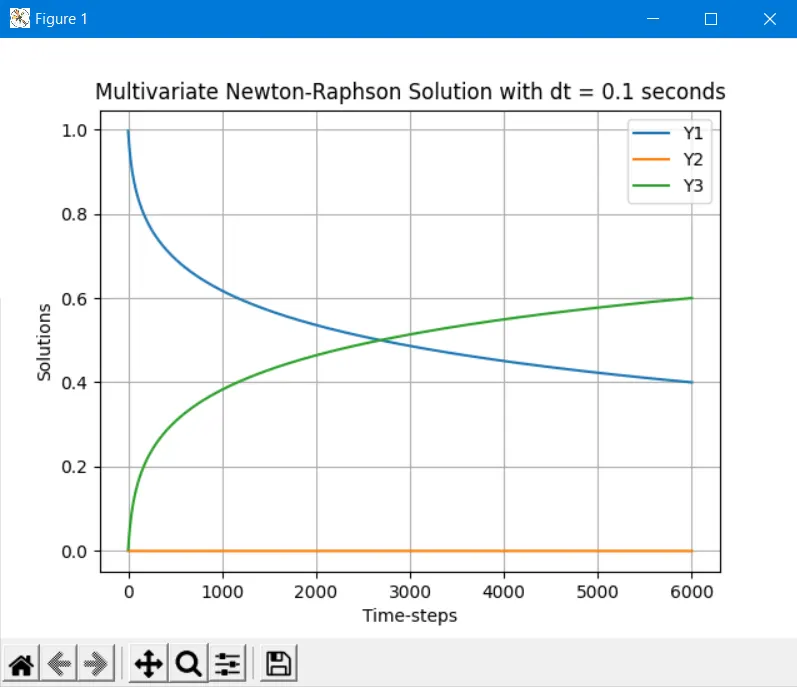

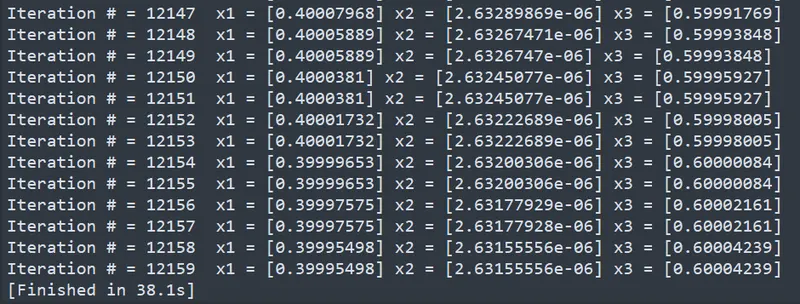
--> We solve a stiff coupled ODE system using an implicit technique. This is important while solving for the species concentration, we have a non-linear coupled stiff ODE system.

--> Implicit systems are stable and relax the time step size chosen.