Week 6 - Multivariate Newton Rhapson Solver
Aim: - To solve following set of Differential equations:
`(dy_1)/dt = -0.04*y_1 + 10^4*y_2*y_3`
`(dy_2)/dt = 0.04*y_1 - 10^4*y_2*y_3 - 3*10^7*y_2^2`
`(dy_3)/dt = 3*10^7*y_2^2`
Objective: -
- Use Multivariate Newton-Rhapson Solver to solve the above set of equation.
- To discuss the step size importance and run the simulation for step sizes [1,0.1,0.01].
Theory: -
The set of equation are coupled with each other so are stiff as one’s values affects the other simultaneously. Implicit method is better suited for such stiff solutions s it provides better stability of solution than other.
Newton-Rhapson Method –
It is a root-finding algorithm which produces successively better approximations to the roots (or zeroes) of a real-valued function.
Let us consider a single-variable function f defined for a real variable x, the function's derivative f ′, and an initial guess x0 for a root of f. Next guess x1 can be calculates by -
`x_1=x_0 - f(x_0 )/(f^' (x_0 ) )`
and successive guess values can be calculated by below formulae until the value reaches acceptable limits or exact value of root.
`x_(n+1)=x_n - f(x_n )/(f^' (x_n ) )`
Multivariate N-R method –
It follows the same approach but can be applied to multiple variables in set of equation. The idea is to start with initial guess values close to the actual roots and form a matrix. A Jacobian Matrix is calculated other with the matrix of root finding equations are set and put into following formulae.
`x_(n ew)=x_(guess)-α . j^(-1).F`
here α is the relaxation factor,
Jacobian Matrix `J = [[(df_1)/(dy_1),(df_1)/(dy_2),(df_1)/(dy_3)],[(df_2)/(dy_1),(df_2)/(dy_2),(df_2)/(dy_3)],[(df_3)/(dy_1),(df_3)/(dy_2),(df_3)/(dy_3)]]`
steps for given equations –
- applying NR method to each equation
`( y_1^n - y_1^(n-1))/dt =-0.04*y_1^n+10^4*y_2^n*y_3^n`
`( y_(2 )^n- y_2^(n-1))/dt=0.04*y_1^n-10^4*y_2^n*y_3^n-3.10^7 (y_2^n )^2`
`( y_(3 )^n- y_3^(n-1))/dt =3.10^7* (y_2^n )^2`
- Rearranging to make it a root finding problem
`y_1^(n-1)+dt*(-0.04*y_1^n+10^4*y_2^n*y_3^n )- y_1^n=0`
`y_2^(n-1)+dt*(0.04*y_1^n-10^4*y_2^n*y_3^n-3.10^7 (y_2^n )^2 )- y_2^n=0`
`y_3^(n-1)+dt*(3.10^7 (y_2^n )^2 )- y_3^n=0`
- The above equations are arranged in a Row vector F and Jacobian is also calculated and re use in the Multivariate NR method.
CODE –
"""
Program to solve Following Set o diferential eqution
 		dy1/dt = -0.04*y1 + 10^4*y2*y3
		dy2/dt = 0.04*y1 - 10^4*y2*y3 - 3*10^7*y2^2
		dy3/dt = 3*10^7*y2^2
using Impicit Multivariate Newton Rhapson
"""

import matplotlib.pyplot as plt
import numpy as np
from numpy.linalg import inv

def f1(y1_old,y1,y2,y3,dt):
	return (y1_old + dt*(-0.04*y1 + y2*y3*pow(10,4)) - y1)

def f2(y2_old,y1,y2,y3,dt):
	return (y2_old + dt*(0.04*y1 - (pow(10,4)*y2*y3) - (3*pow(10,7)*pow(y2,2))) - y2)

def f3(y3_old,y1,y2,y3,dt):
	return (y3_old + dt*(3*pow(10,7)*pow(y2,2)) - y3)

def j(y1_old,y2_old,y3_old,y1,y2,y3,dt):

	j=np.ones((3,3))  # assigning 3*3 matrix to j with 1
	h = 1e-6        # step size

	j[0,0] = (f1(y1_old,y1+h,y2,y3,dt) - f1(y1_old,y1,y2,y3,dt))/h
	j[0,1] = (f1(y1_old,y1,y2+h,y3,dt) - f1(y1_old,y1,y2,y3,dt))/h
	j[0,2] = (f1(y1_old,y1,y2,y3+h,dt) - f1(y1_old,y1,y2,y3,dt))/h

	j[1,0] = (f2(y2_old,y1+h,y2,y3,dt) - f2(y2_old,y1,y2,y3,dt))/h
	j[1,1] = (f2(y2_old,y1,y2+h,y3,dt) - f2(y2_old,y1,y2,y3,dt))/h
	j[1,2] = (f2(y2_old,y1,y2,y3+h,dt) - f2(y2_old,y1,y2,y3,dt))/h

	j[2,0] = (f3(y3_old,y1+h,y2,y3,dt) - f3(y3_old,y1,y2,y3,dt))/h
	j[2,1] = (f3(y3_old,y1,y2+h,y3,dt) - f3(y3_old,y1,y2,y3,dt))/h
	j[2,2] = (f3(y3_old,y1,y2,y3+h,dt) - f3(y3_old,y1,y2,y3,dt))/h

	return j

# assining values to initial guess values

y1_old = 1
y2_old = 0
y3_old = 0

# defining a matrix with initial guess values
y_old = np.ones((3,1))
y_old[0] = y1_old
y_old[1] = y2_old
y_old[2] = y3_old

F = np.copy(y_old)

# parameters for NR method


dt = 1
t = np.arange(0,600,dt)

# defining the function variable and iteration
y1 = []
y2 = []
y3 = []
iteration = []

cntr = 1

for i in range(0,len(t)):

	# initilising error
	err = 9e9
	tol = 1e-6

	while (err > tol):

		# calling jacobian function j
		J = j(y1_old,y2_old,y3_old,y_old[0],y_old[1],y_old[2],dt)

		# defining Functon vector F

		F[0] = f1(y1_old,y_old[0],y_old[1],y_old[2],dt)
		F[1] = f2(y2_old,y_old[0],y_old[1],y_old[2],dt)
		F[2] = f3(y3_old,y_old[0],y_old[1],y_old[2],dt)

		# calculating new values
		y_new = y_old - np.matmul(inv(J),F)

		# calculating error
		err = np.max(np.abs(y_new-y_old))

		# print('error = %d ' %err)

		# updating old values with new
		y_old = y_new

	message = 'iter No. = {0} y1 = {1} y2 = {2} y3 = {3} Max error = {4}'.format(cntr , y_new[0], y_new[1], y_new[2], err)

	print(message)

	# incrementing in counter
	cntr = cntr + 1

	y1.append(y_new[0])
	y2.append(y_new[1])
	y3.append(y_new[2])

	iteration.append(cntr)

	# updating old values with new
	y_old = y_new
	y1_old = y_new[0]
	y2_old = y_new[1]
	y3_old = y_new[2]


plt.plot(iteration,y1,color = 'r')
plt.plot(iteration,y2,color = 'g')
plt.plot(iteration,y3,color = 'b')
plt.xlabel('Number of steps')
plt.ylabel('Variables(Species)')
plt.grid ('on')
plt.legend(['y1','y2','y3'])
plt.title('Multivariate Newton Raphson Method for time step = %f sec' %dt)
plt.show()
Results: -
1. For time step = 1 sec
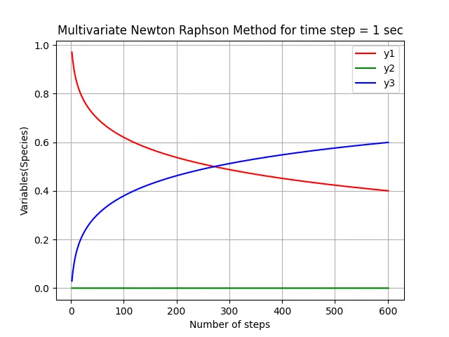
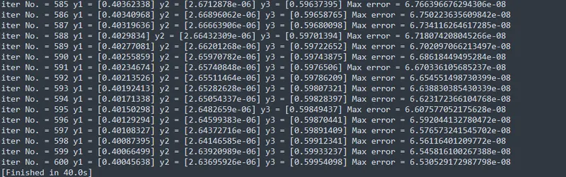
Time taken for solution = 40 sec
2. For time step dt = 0.1 sec
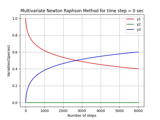
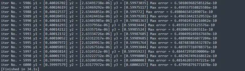
Time taken for solution = 34.1 sec
3. For time step dt = 0.01
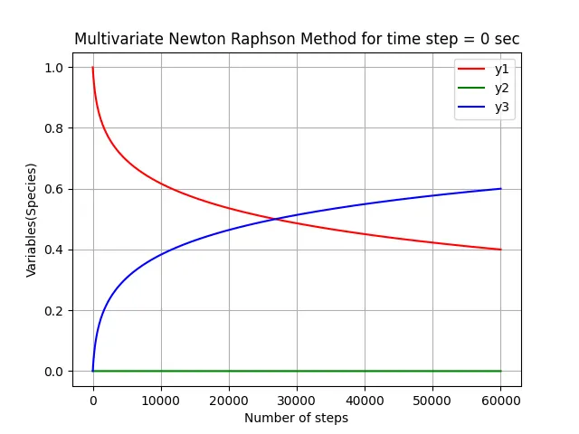
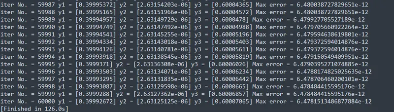
Time taken for solution = 126 sec
Conclusion: -
1. Each time step gives similar result.
2. The time taken to solve for each time step is different where for dt = 0.1 the solution is fastest
Selection of time step -
Seecting time step is on o the major parameter which can affect the code drastically. Lowet time step some time consume much more time then required AS here time step 0.01 take 126 sec which is lready three time than other.
Whereas if time step is larger it could fail to capture the appropriate simulation and can produce unreal results. Hence selecting proper time step can minimize the calculation time without compromising the result as here 0.1 sec stand out than other two by providing more precise result with less time consumption.