Week 6 - Multivariate Newton Rhapson Solver

Aim: To perform the Multivariate Newton Rhapson technique to solve the set of equations provided and choose the suitable timestep

Introduction:

The Newton-Raphson method is a quick way to find a good approximation for the root of a real-valued function. This method works for any equation, polynomial or not, as long as the function is differentiable in the desired interval. 's often become increasingly better approximations of the function's root. The multivariate newton raphson method is used to solve the coupled equations. Newton raphson method is the iteration of the guess values to get the required accurate solutions.

Jacobian matrix is used to store all the possible derivatives of the coupled equations. Backward differencing method(Implicit) is used for improving the previous solution. As it is unconditionally stable irrespective of the time step.

The set of equations given to be solve

`(dy_1)/(dt) = -0.04y_1 + 10^4y_2y_3`

`(dy_2)/(dt) = 0.04y_1 - 10^4y_2y_3 - 3*10^7*y_2^(2)`

`(dy_3)/(dt) = 3*10^7*y_2^(2)`

The solving of equations to input into the code

Backward difference method /Implicit Form

`f_1 = y_1^n + h(-0.04y_1 + 10^4y_2y_3) -y_1^(n-1) = 0`

`f_2 =y_2^n+ h(0.04y_1^n - 10^4y_2^ny_3^n - 3*10^7*(y_2^n)^(2))-y_2^(n-1)= 0`

`f3 = y_3^n +3*10^7*(y_2^n)^2 -y_3^(n-1) =0`

Jacobian matrix

`[[{partialf_1^n}/{partialy_1^n},{partialf_1^n}/{partialy_2^n},{partialf_1^n}/{partialy_3^n}],[{partialf_2^n}/{partialy_1^n},{partialf_2^n}/{partialy_2^n},{partialf_2^n}/{partialy_3^n}],[{partialf_3^n}/{partialy_1^n},{partialf_3^n}/{partialy_2^n},{partialf_3^n}/{partialy_3^n}]]`

Newton raphson solver to solve coupled equations using imlicit method

`y(New)^n =y_(old)^n + alpha[(J^-1)F]^n`

F is a column matrix with all the three expressions incorporated

`F =[[f_1],[f_2],[f_3]]`

Given conditions:

Use implicit Euler Method/Backward Differencing, and assume the initial conditions as 1 for y1 and 0 for y2 and y3 respectively. The simulation time is 10 minutes.

Code steps:

Required modules and libraries are imported. Then the time constraints are defined along with the time step. After that Equations are defined and the jacobian matrix is defined. Each element of the jacobian matrix is defined. Initial guess values are defined and the F vector is defined. Tolerance and error values are defined, and old values are also stored. for loop is initiated to loop for all the n time steps, while loop is used to know if the error is less than the tolerance. Jacobian is called and F column vectors are also defined. Newton raphson solver is used to solve for the roots. Error is calculated and the old value of y is updated. The n plotting is done.

Python code:

"""Multivariate Newton Raphson Method
"""
import math
import matplotlib.pyplot as plt
import numpy as np
from numpy.linalg import inv

#Time considerations
t_start = 0
t_end = 600
n = 60000
dt = (t_end-t_start)/n

# Equation
def f1(y1_old,y2_old,y3_old,y1,y2,y3,dt):
	return (y1_old + (-0.04*y1 + pow(10,4)*y2*y3)*dt -y1)

def f2(y1_old,y2_old,y3_old,y1,y2,y3,dt):
	return (y2_old + (0.04*y1 -pow(10,4)*y2*y3 -3*pow(10,7)*pow(y2,2))*dt -y2)

def f3(y1_old,y2_old,y3_old,y1,y2,y3,dt):
	return (y3_old + dt*(3*pow(10,7)*pow(y2,2))-y3)

def jacobian(y1_old,y2_old,y3_old,y1,y2,y3,dt):

	j = np.ones((3,3))
	h = 1e-5

	j[0,0] = (f1(y1_old,y2_old,y3_old,y1+h,y2,y3,dt)-f1(y1_old,y2_old,y3_old,y1,y2,y3,dt))/h
	j[0,1] = (f1(y1_old,y2_old,y3_old,y1,y2+h,y3,dt)-f1(y1_old,y2_old,y3_old,y1,y2,y3,dt))/h
	j[0,2] = (f1(y1_old,y2_old,y3_old,y1,y2,y3+h,dt)-f1(y1_old,y2_old,y3_old,y1,y2,y3,dt))/h

	j[1,0] = (f2(y1_old,y2_old,y3_old,y1+h,y2,y3,dt)-f2(y1_old,y2_old,y3_old,y1,y2,y3,dt))/h
	j[1,1] = (f2(y1_old,y2_old,y3_old,y1,y2+h,y3,dt)-f2(y1_old,y2_old,y3_old,y1,y2,y3,dt))/h
	j[1,2] = (f2(y1_old,y2_old,y3_old,y1,y2,y3+h,dt)-f2(y1_old,y2_old,y3_old,y1,y2,y3,dt))/h

	j[2,0] = (f3(y1_old,y2_old,y3_old,y1+h,y2,y3,dt)-f3(y1_old,y2_old,y3_old,y1,y2,y3,dt))/h
	j[2,1] = (f3(y1_old,y2_old,y3_old,y1,y2+h,y3,dt)-f3(y1_old,y2_old,y3_old,y1,y2,y3,dt))/h
	j[2,2] = (f3(y1_old,y2_old,y3_old,y1,y2,y3+h,dt)-f3(y1_old,y2_old,y3_old,y1,y2,y3,dt))/h

	return j

#initial guess values
y1_old =1
y2_old =0
y3_old =0

error=9e9

Y_old = np.ones((3,1))
Y_old[0] = y1_old
Y_old[1] = y2_old
Y_old[2] = y3_old

#F vector
F = np.copy(Y_old)

#tolerance
tol = 1e-6
alpha =1
y_1 =[]
y_2 =[]
y_3 =[]
iteration = []

#looping
iter = 1

for i in range (0,n):
	while error > tol:
		j = jacobian(y1_old,y2_old,y3_old,Y_old[0],Y_old[1],Y_old[2],dt)

		#computing F vector
		F[0] = f1(y1_old,y2_old,y3_old,Y_old[0],Y_old[1],Y_old[2],dt)
		F[1] = f2(y1_old,y2_old,y3_old,Y_old[0],Y_old[1],Y_old[2],dt)
		F[2] = f3(y1_old,y2_old,y3_old,Y_old[0],Y_old[1],Y_old[2],dt)

		#new values
		Y_new = Y_old - alpha*np.matmul(inv(j), F)

		#Error calculation
		error = np.max(np.abs(Y_new-Y_old))
		print(error)

		#Updating old values
		Y_old = Y_new;

	#log message
	log_message = 'iteration number = {0} y1 = {1} y2 = {2} y3 = {3}'.format(iter, Y_new[0], Y_new[1], Y_new[2])
	print(log_message)

	iter = iter+1

	#Appending for plotting
	y_1.append(Y_new[0])
	y_2.append(Y_new[1])
	y_3.append(Y_new[2])
	
	iteration.append(iter)

	Y_old = Y_new
	y1_old = Y_new[0]
	y2_old = Y_new[1]
	y3_old = Y_new[2]

	error = 9e9
#plotting
plt.plot(iteration,y_1,color='grey')
plt.plot(iteration,y_2,color='cyan')
plt.plot(iteration,y_3,color='pink')
plt.xlabel('dt')
plt.ylabel('Variable')
plt.grid ('on')
plt.legend(['y_1','y_2','y_3'])
plt.title('Multivariate Newton Raphson Method for dt = 0.01')
plt.show()

codes for both the plots are the same except the n value

Plots

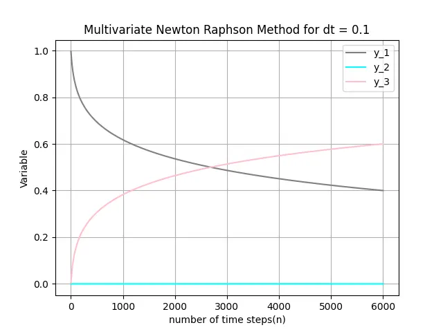
Plot with dt 0.1

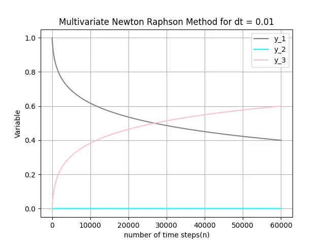
Plot with dt 0.01

conclusion:

• There is no significant variation in the plots with change in the dt.
• As the solving method of newton raphson method is implicit the solution is unconditionally stable irrespective of the time step.
• With the decreasing time step the simulation time increases and if the time step is large simulation time is drastically reduced.
• Implicit methods are stable at any time step the accuracy comes in the smaller time steps, the time took for simulating dt 0.1 is smaller than the dt 0.01.
• ideal time step varies from problem to problem it depends on the time available accuracy of the solution needed and the computational power. In this case, a smaller time step is preferred.