Week 6 - Multivariate Newton Rhapson Solver

MULTIVARIATE NEWTON RAPHSON SOLVER

AIM: To write a code and solve the equation given by multivariate Newton Raphson solver.

OBJECTIVE:

• you will solve the set of equations given below,

• Get the code working as shown in the video
• Incorporate numerical jacobian. That is, the jacobian should be estimated numerically and not analytically.

• Solve the problem using Implicit Euler Method/Backward Differencing, assume the initial conditions as 1 for y1 and 0 for y2 and y3 respectively.

• Take alpha as 1. Run the simulation for 10 minutes.

• Choose a suitable step size and explain the reason for choosing that step size, what is the ideal step size in this case?

• Paste the code a report and the results, lack of attaching the requested item will result in a points deduction

THEORY:

The Newton Raphson method is implemented for each time step set for the given simulation time. The difference is that, in Multivariate, the approximations are calculated in a matrix form as there is more than one unknown. The general principle for the Multivariate Newton Rapson is given below:

`X_(n+1) = X_n - alpha*J^-1*F`

where `X_n` is the old value

`X_(n+1)` is the new value which we are guessing with respect to the old value,

`alpha` is the relaxation factor,

`J^-1` is the inverse Jacobian matrix and

`F` is a matrix that contains the given system of equations.

The matrix representation of the above principle is given below:

*In the above figure, `alpha` is multiplied to the Jacobian inverse and the function matrix term.

Jacobian Matrix has been calculated numerically as:

`(df_i)/dx_j = (f(x_j+h) - f(x_j))/h`

We are also using the Implicit Euler or otherwise known as the Backward Differencing method for the outer time integration loop for this challenge.

The Backward Differencing method is a finite approximation method that uses the function values at x and x − i where i is the step size. The general principle for this method is mentioned below:

`f'(x) = (f(x)- f(x-h))/h`

Given the step size (h), note that this formula uses the values at the current time step and the point at the previous step. As it moves in the backward direction, it is called the backward difference method.

The given initial conditions for the unknowns are: -

y1 = 1

y2 = 0

y3 = 0

The simulation run time is 10 min = 600 seconds

Here, we are initializing the ODE in the form:

`f'(x) = x_("old value") + dt*f(x) - x_("new value")`

The general layout of the code is given below:

• Outer Time Integration Loop
• Assembling the ODE System
• Newton Raphson solver till convergence
• Get new values and update them
• End of Outer Loop

CODE AND SOLUTION:

Program to solve a multivariate system using Newton Raphson solver.

import numpy as np 
import matplotlib.pyplot as plt
from numpy.linalg import inv

# Functions 
def f1(y1,y2,y3,y_old1,dt): 
	return y_old1 + dt*(-0.04*y1 + (pow(10,4)*y2*y3)) - y1

def f2(y1,y2,y3,y_old2,dt): 
	return y_old2 + dt*(0.04*y1 - (pow(10,4)*y2*y3) - (3*pow(10,7)*pow(y2,2))) - y2

def f3(y1,y2,y3,y_old3,dt): 
	return y_old3 + dt*(3*pow(10,7)*pow(y2,2)) - y3

def jacobian(y_new,y_old,dt):

	# Identity 3x3 matrix
	J = np.ones((3,3))

	# Using dummy values
	y1 = y_new[0] 
	y2 = y_new[1] 
	y3 = y_new[2] 

	
	y_old1 = y_old[0]
	y_old2 = y_old[1]
	y_old3 = y_old[2]

	dy = 1e-10

	J[0,0] = (f1(y1+dy,y2,y3,y_old1,dt) - f1(y1,y2,y3,y_old1,dt))/dy
	J[0,1] = (f1(y1,y2+dy,y3,y_old1,dt) - f1(y1,y2,y3,y_old1,dt))/dy
	J[0,2] = (f1(y1,y2,y3+dy,y_old1,dt) - f1(y1,y2,y3,y_old1,dt))/dy

	J[1,0] = (f2(y1+dy,y2,y3,y_old1,dt) - f2(y1,y2,y3,y_old1,dt))/dy
	J[1,1] = (f2(y1,y2+dy,y3,y_old1,dt) - f2(y1,y2,y3,y_old1,dt))/dy
	J[1,2] = (f2(y1,y2,y3+dy,y_old1,dt) - f2(y1,y2,y3,y_old1,dt))/dy

	J[2,0] = (f3(y1+dy,y2,y3,y_old1,dt) - f3(y1,y2,y3,y_old1,dt))/dy
	J[2,1] = (f3(y1,y2+dy,y3,y_old1,dt) - f3(y1,y2,y3,y_old1,dt))/dy
	J[2,2] = (f3(y1,y2,y3+dy,y_old1,dt) - f3(y1,y2,y3,y_old1,dt))/dy

	return J

# Backward differencing
y_old = np.zeros((3,1))
y_old[0] = 1

y_new = np.zeros((3,1))

F = np.copy(y_new)

a = 1 
tol = 1e-10
error = 1e9
dt = 1
# time to run simulation = 10 mins = 600 secs
t = np.arange(0,600,dt)
e = np.zeros((int(600/dt),1))
Y1 = np.zeros((int(600/dt),1))
Y2 = np.zeros((int(600/dt),1))
Y3 = np.zeros((int(600/dt),1))

for i in range(0,len(t)):
	y_old1 = y_old[0]
	y_old2 = y_old[1]
	y_old3 = y_old[2]
	y_guess = np.copy(y_old)

	while error > tol:

		J = jacobian(y_new,y_old,dt)

		y1g = y_guess[0]
		y2g = y_guess[1]
		y3g = y_guess[2]

		F[0] = f1(y1g,y2g,y3g,y_old1,dt)
		F[1] = f2(y1g,y2g,y3g,y_old2,dt)
		F[2] = f3(y1g,y2g,y3g,y_old3,dt)

		y_new = y_guess - a*np.matmul(inv(J),F)
		error = max(abs(y_new-y_guess))

		y_guess = y_new
	

	e[i] = error
	y_old = y_new
	Y1[i] = y_new[0]
	Y2[i] = y_new[1]
	Y3[i] = y_new[2]
	error = 1e9


plt.plot(t,Y1, label = 'y1')
plt.plot(t,Y2, label = 'y2')
plt.plot(t,Y3, label = 'y3')
plt.title('Multi-variate Newton Raphson Solver for dt = ' +str(dt))
plt.xlabel('Number of time steps')
plt.ylabel('Variables')
plt.legend()
plt.grid()
plt.show()

The error and initial values are defined before the time loop starts and are accordingly updated at the end of the loop for the next iteration to take place.

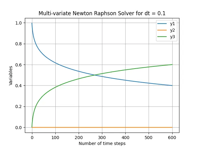
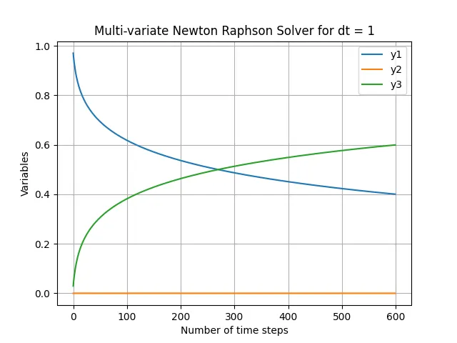
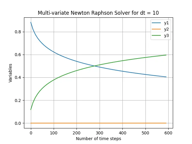
CONCLUSION:

For the time step dt, if we take dt as 1, there are 600 steps in the system and hence results are sharp and not that accurate. But if we give a smaller dt of say, 1e-2, we have too many iterations to complete in an already complex multivariate solver, even though the solution result comes out smooth. Hence, an average dt value of 0.1 is assumed in this case to give an accurate representation of data and also sufficiently time efficient. The results show the variations in values and their domains getting smaller due to an increase in time step size. Hence the ideal time step for this case is assumed to be 0.1.