Week 6 - Multivariate Newton Rhapson Solver

Aim

To solve ODE's using multivariant Newton Raphson method

Introduction

The Newton Raphson method is used to get the solutions of nonlinear coupled equations system. The Newton-Raphson method (also known as Newton's method) is a way to find an approximation for the root of a real-valued function f(x)=0">f(x)=0. The method rely on the idea that a continuous and differentiable function can be approximated by a straight-line tangent to it.

Following ODE's are to be solved using Newton Raphson method

dy₁/dt = -0.04y₁ + 10⁴y₂y₃

dy₂/dt = 0.04y₁ - 10⁴y₂y₃-3 * 10⁷y₂2

dy₃/dt = 3* 10⁷y₂²

we have initial guess values:

y1=1

y2=0

y3=0

For all of the below equation superscript 'n' shows new node or new timestep while 'n-1' shows previous or old timestep or node.

By using BDM,

yⁿ-y^n-1 / Δt = C

yⁿ - (Δt×C) = y^n-1

So above ODE's can be calculated as,

y₁ⁿ-y_1^n-1 / Δt = (-0.04y₁ + 10⁴y₂y₃)ⁿ

y₂ⁿ-y₂^n-1 / Δt = (0.04y₁ - 10⁴y₂y₃-3 * 10⁷y₂^2)ⁿ

y₃ⁿ-y₃^n-1 / Δt = (3* 10⁷y₂²)ⁿ

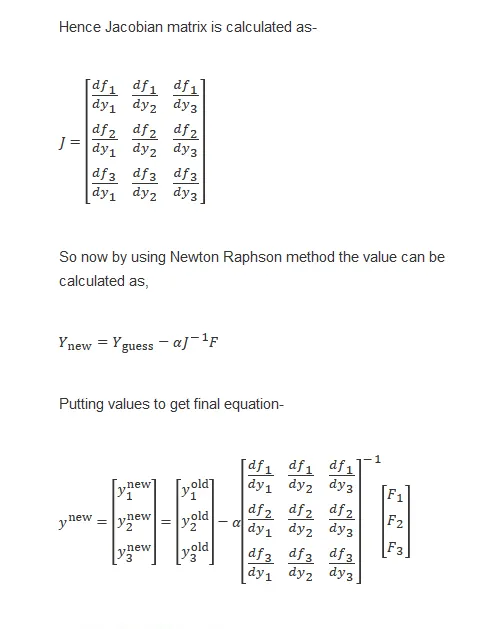
Hence we get system of linear equations,

F₁ⁿ => y_1^n-1 +(Δt) (-0.04y₁ + 10⁴y₂y₃)ⁿ -y₁ⁿ=0

F₂ⁿ => y₂^n-1 +(Δt) (0.04y₁ - 10⁴y₂y₃-3 * 10⁷y₂2)ⁿ -y₂ⁿ=0

F₃ⁿ => y₃^n-1 +(Δt) (3* 10⁷y₂²)ⁿ -y₃ⁿ=0

NOTE:

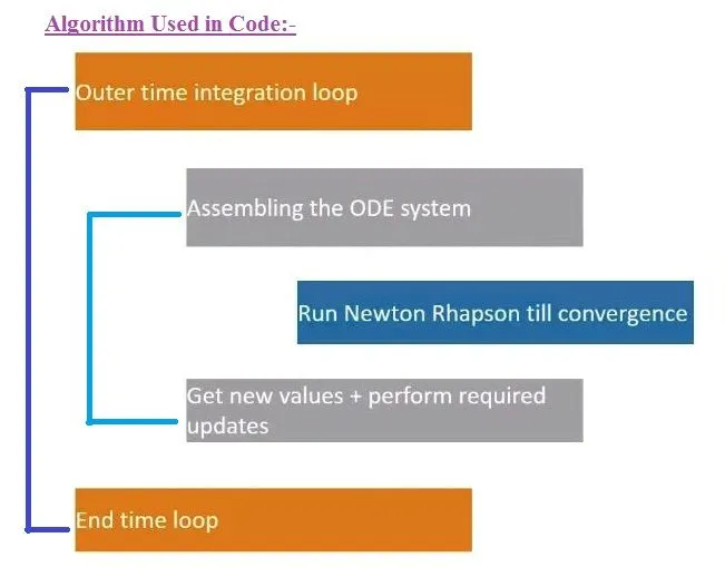
For solving the actual problem using Python, we proceed as usual and solve the quadratic equations first by defining functions for each equation. An arbitraty dy value is assumed for the accurate discretization of the PDE. In this case, dy = 1e-10.

Guess values are assumed as an array which will be used in the time loop required for the problem. We simulate the system for 10 mins, i.e, for 600 seconds.

import numpy as np 
import matplotlib.pyplot as plt
from numpy.linalg import inv

# Functions to solve each multivariable equation(as shown above)
def f1(y1,y2,y3,y_old1,h): 
	return y_old1 + h*(-0.04*y1 + (pow(10,4)*y2*y3)) - y1

def f2(y1,y2,y3,y_old2,h): 
	return y_old2 + h*(0.04*y1 - (pow(10,4)*y2*y3) - (3*pow(10,7)*pow(y2,2))) - y2

def f3(y1,y2,y3,y_old3,h): 
	return y_old3 + h*(3*pow(10,7)*pow(y2,2)) - y3

# function for the jacobian matrix 
def jacobian(y_new,y_old,h):

	# input an identity 3x3 matrix
	J = np.ones((3,3))

	# Using guess values that will be updated for each time step when solving
	y1 = y_new[0] 
	y2 = y_new[1] 
	y3 = y_new[2] 

	# Old values are the input guess values we give
	y_old1 = y_old[0]
	y_old2 = y_old[1]
	y_old3 = y_old[2]

	# To solve the system numerically
	dy = 1e-10

	J[0,0] = (f1(y1+dy,y2,y3,y_old1,h) - f1(y1,y2,y3,y_old1,h))/dy
	J[0,1] = (f1(y1,y2+dy,y3,y_old1,h) - f1(y1,y2,y3,y_old1,h))/dy
	J[0,2] = (f1(y1,y2,y3+dy,y_old1,h) - f1(y1,y2,y3,y_old1,h))/dy

	J[1,0] = (f2(y1+dy,y2,y3,y_old1,h) - f2(y1,y2,y3,y_old1,h))/dy
	J[1,1] = (f2(y1,y2+dy,y3,y_old1,h) - f2(y1,y2,y3,y_old1,h))/dy
	J[1,2] = (f2(y1,y2,y3+dy,y_old1,h) - f2(y1,y2,y3,y_old1,h))/dy

	J[2,0] = (f3(y1+dy,y2,y3,y_old1,h) - f3(y1,y2,y3,y_old1,h))/dy
	J[2,1] = (f3(y1,y2+dy,y3,y_old1,h) - f3(y1,y2,y3,y_old1,h))/dy
	J[2,2] = (f3(y1,y2,y3+dy,y_old1,h) - f3(y1,y2,y3,y_old1,h))/dy

	return J

# Input the guess values as old, due to use of backward differencing
y_old = np.zeros((3,1))
y_old[0] = 1

y_new = np.zeros((3,1))

# numpy column vector for F matrix
F = np.copy(y_new)

# inputs
a = 1 # alpha for Newton raphson solver(given in problem statement)
tol = 1e-10
error = 1e9

dt = 0.1 # time step
h = dt

# simulation time = 10 mins = 600 secs
t = np.arange(0,600,h)# divide 600 secs in h time steps

# Empty arrays initialized for storing final values
e = np.zeros((int(600/h),1))
Y1 = np.zeros((int(600/h),1))
Y2 = np.zeros((int(600/h),1))
Y3 = np.zeros((int(600/h),1))

# time loop started
for i in range(0,len(t)):
	y_old1 = y_old[0]
	y_old2 = y_old[1]
	y_old3 = y_old[2]
	y_guess = np.copy(y_old)

	while error > tol:
		# computing jacobian - old values used
		J = jacobian(y_new,y_old,h)

		y1g = y_guess[0]
		y2g = y_guess[1]
		y3g = y_guess[2]

		# Computing F vector - old values used
		F[0] = f1(y1g,y2g,y3g,y_old1,h)
		F[1] = f2(y1g,y2g,y3g,y_old2,h)
		F[2] = f3(y1g,y2g,y3g,y_old3,h)

		# computing new values
		y_new = y_guess - a*np.matmul(inv(J),F)
		error = max(abs(y_new-y_guess))

		y_guess = y_new
	
	# Values after each time step added into array
	e[i] = error
	y_old = y_new
	Y1[i] = y_new[0]
	Y2[i] = y_new[1]
	Y3[i] = y_new[2]

	error = 1e9

# Plots
plt.plot(t,Y1, label = 'y1')
plt.plot(t,Y2, label = 'y2')
plt.plot(t,Y3, label = 'y3')
plt.title('Multi-variate Newton Raphson Solver for dt = ' +str(h))
plt.xlabel('Time (secs)')
plt.ylabel('$y_i$')
plt.legend()
plt.grid()
plt.show()

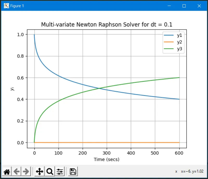
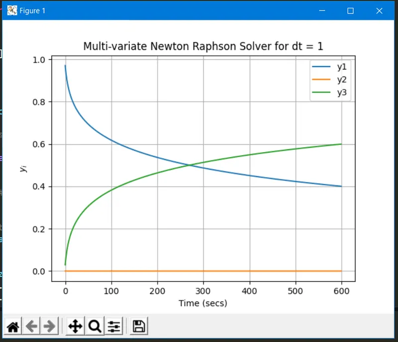
PLOTS

Observations:

i) Change in time step doesn't make any big difference in final solution.

ii) Small value of time step takes longer time (iterations) to converged result which may increase cost.

iii) Hence, an average dt value of 0.1 is assumed in this case to give an accurate representation of data and also sufficiently time efficient.