Week 6 - Multivariate Newton Rhapson Solver

Aim:Solving the set of ordinary differential equation using multivariate newton raphson method.

Objective:

• Solving the set of ordinary differential equation using Implicit Euler Method/forward Differencing.Run the simulation for 10 minutes
• Plot the number of iteration and values for variable y1,y2, an y3.

Introduction:

In newton raphson method we assume intial value for co-efficient and apply a technique to calculate approximate values of the roots.

But the newton raphson method is applicable only for single ODE.

If we have system of ODE's how we can solve??

Here comes a modification of newton raphson method the Multivariate newton raphson method, In this method we can solve multiple number of ODE's together.

Where is it useful??

The major use is to calculate the rate of change of each species in the no of reactions during combustion process.

The Coupled ODE's given are:-

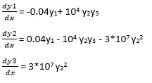
To solve this equation by using backward differencing we can modify them as:

Y₁ⁿ = y₁^n-1 + (-0.04y₁ⁿ + 10⁴ y₂ⁿ y₃ⁿ)*∆t

Y₂ⁿ = y₂^n-1 + (0.04y₁ⁿ - 10⁴ y₂ⁿ y₃ⁿ - 3*10⁷ y₂²ⁿ )*∆t

Y₃ⁿ = y₃^n-1 + (3*10⁷ y₂²ⁿ )*∆t

This are the equation converted into backward differencing scheme

Next step is to calculate Jacobian matrix, to calculate Jacobian matrix we should consider number of functions and no of co-efficient in each function whose values to be determined.

In above problems we have 3 functions and 3 co-efficient/variables in each equation which turns our Jacobian matrix into 3*3 matrix.

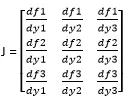
We must use backward differencing scheme here to calculate each values i.e.

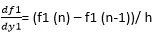
We can also apply backward and central differencing scheme to check the values and compare which scheme is suitable.

Once we have calculated the value of Jacobian and function now we can use multivariate newton Raphson technique, to calculate the value of y1, y2, and y3.

Y_new = Y_old – α*J^-1*F

Where,

Steps/logic of the program:

• The step 1 is to define the function to return the values of ODE's.
• Calculate the Jacobian matrix using above logic.
• Define initial guess for all variables,assume the initial conditions as 1 for y1 and 0 for y2 and y3 respectively.
• Create a loop to calculate values of variables usin multivariate newton raphson
• Plot the number of iterations and variation of variables.

Python code for solving the system of ODE's using multivariate newton raphson method:

import math
import numpy as np 
from numpy.linalg import inv
import matplotlib.pyplot as plt 

#defining the functions
def f1(y1_old,y1,y2,y3,dt):
	return (y1_old + dt*(-0.04*y1 + y2*y3*1e4) - y1)

def f2(y2_old,y1,y2,y3,dt):
	return (y2_old + dt*(0.04*y1 - (1e4*y2*y3) -(3e7*y2*y2)) -y2)	

def f3(y3_old,y1,y2,y3,dt):
	return (y3_old + dt*(3e7*y2*y2) - y3)	
	
#Function for calculation of jacobian
def jacobian(y1_old,y2_old,y3_old,y1,y2,y3,dt):
	J = np.ones((3,3))	

	#step size
	h= 1e-8
	J[0,0] = (f1(y1_old,y1+h,y2,y3,dt) - f1(y1_old,y1-h,y2,y3,dt))/(2*h)
	J[0,1] = (f1(y1_old,y1,y2+h,y3,dt) - f1(y1_old,y1,y2-h,y3,dt))/(2*h)
	J[0,2] = (f1(y1_old,y1,y2,y3+h,dt) - f1(y1_old,y1,y2,y3-h,dt))/(2*h)

	J[1,0] = (f2(y2_old,y1+h,y2,y3,dt) - f2(y2_old,y1-h,y2,y3,dt))/(2*h)
	J[1,1] = (f2(y2_old,y1,y2+h,y3,dt) - f2(y2_old,y1,y2-h,y3,dt))/(2*h)
	J[1,2] = (f2(y2_old,y1,y2,y3+h,dt) - f2(y2_old,y1,y2,y3-h,dt))/(2*h)

	J[2,0] = (f3(y3_old,y1+h,y2,y3,dt) - f3(y3_old,y1-h,y2,y3,dt))/(2*h)
	J[2,1] = (f3(y3_old,y1,y2+h,y3,dt) - f3(y3_old,y1,y2-h,y3,dt))/(2*h)
	J[2,2] = (f3(y3_old,y1,y2,y3+h,dt) - f3(y3_old,y1,y2,y3-h,dt))/(2*h)		

	return J

#initial assumption
y1_old = 1
y2_old = 0
y3_old = 0	


#inputs
error = 9e9
tol = 1e-6
alpha = 1
t_start = 0
t_end = 600
n=6001
t = np.linspace(t_start,t_end,n)
dt = 0.1
iteration = []
iter = 1
error_new=[]
y_1 = []
y_2 = []
y_3 = []

y_old = np.ones((3,1))
y_old[0]=y1_old;
y_old[1]=y2_old;
y_old[2]=y3_old;

#initial function matrix
F = np.copy(y_old)

#loop for multivariate newton raphson method
for i in range(0,len(t)):
	error = 9e9
	while (error > tol):
		J = jacobian(y1_old,y2_old,y3_old,y_old[0],y_old[1],y_old[2],dt);
		
		F[0] = f1(y1_old,y_old[0],y_old[1],y_old[2],dt)
		F[1] = f2(y2_old,y_old[0],y_old[1],y_old[2],dt)
		F[2] = f3(y3_old,y_old[0],y_old[1],y_old[2],dt)

		y_new = y_old - alpha*np.matmul(inv(J),F)
		error = np.max(np.abs(y_new - y_old))
		y_old = y_new

	logmessage = 'iteration number = {0} y1 = {1} y2 = {2} y3 = {3}'.format(iter,y_new[0],y_new[1],y_new[2])
	print(logmessage)
	y_1.append(y_new[0])
	y_2.append(y_new[1])
	y_3.append(y_new[2])

	iter = iter + 1
	iteration.append(iter)
	y1_old=y_new[0]
	y2_old=y_new[1]
	y3_old=y_new[2]

#plotting
plt.plot(iteration,y_1,label = 'y1')
plt.plot(iteration,y_2,label = 'y2')
plt.plot(iteration,y_3,label = 'y3')
plt.xlabel('No of iterations')
plt.ylabel('value for variables')
plt.legend(loc = 'best')
plt.show()

PLOT:

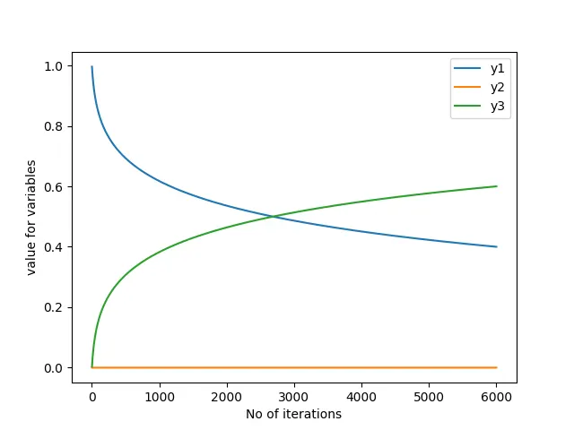
Plot shows the values of unknows variables with no of iteration it takes to get closer to accurate solution.

OUTPUT:

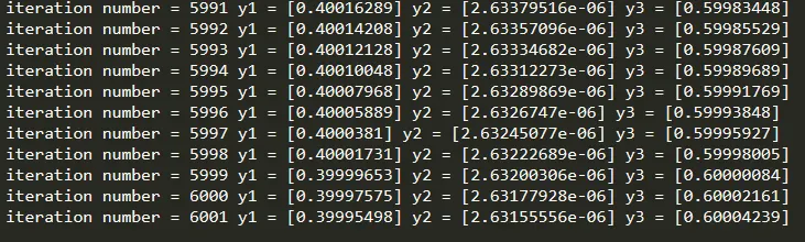
The number of iteration is calculated based on the time given for simulation and the time step.

Choose a suitable step size and explain the reason for choosing that step size, what is the ideal step size in this case?

The step size values can be choosed based on no of iterations we want to run for a particular problem, as step size decreases the number of iteration increases and also the accuracy increases and the solution is stable.

In my program I used step size of 0.1 which tends to 6001 iterations, If I take step size to 0.01 the number of iteration increases to 60001.Depending upon how stiff we need our solution process to be we can use different step size.

For above problem the step size of 0.1 is precise, we can also run a step size of 1,10 if we know that particular problem doesn't need a amount of stiffness which in turn will reduce the simulation time.