Week 6 Fuel cell powered vehicle model

Make a MATLAB model of fuel cell-powered electric vehicle and comment on results

A fuel cell is a device that generates electricity by a chemical reaction. Every fuel cell has two electrodes called, respectively, the anode and cathode. The reactions that produce electricity take place at the electrodes. Every fuel cell also has an electrolyte, which carries electrically charged particles from one electrode to the other, and a catalyst, which speeds the reactions at the electrodes.

Hydrogen is the basic fuel, but fuel cells also require oxygen. One great appeal of fuel cells is that they generate electricity with very little pollution–much of the hydrogen and oxygen used in generating electricity ultimately combine to form a harmless byproduct, namely water.

The Fuel Cell in Electric Vehicles

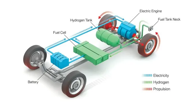
Like all-electric vehicles, fuel cell electric vehicles (FCEVs) use electricity to power an electric motor. In contrast to other electric vehicles, FCEVs produce electricity using a fuel cell-powered by hydrogen, rather than drawing electricity from only a battery. During the vehicle design process, the vehicle manufacturer defines the power of the vehicle by the size of the electric motor(s) that receive electric power from the appropriately sized fuel cell and battery combination.

Although automakers could design an FCEV with plug-in capabilities to charge the battery, most FCEVs today use the battery for recapturing braking energy, providing extra power during short acceleration events, and to smooth out the power delivered from the fuel cell with the option to idle or turn off the fuel cell during low power needs. The amount of energy stored on board is determined by the size of the hydrogen fuel tank. This is different from an all-electric vehicle, where the amount of power and energy available are both closely related to the batteries.

MATLAB Modeling of fuel cell-powered electric vehicle

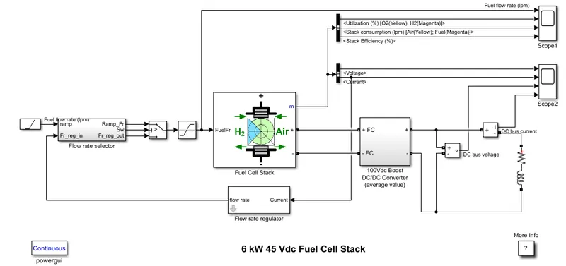
Step 1: Open "power_fuel_cell" model.

Step 2: Change input

Here as we can see a ramp signal is given as load reference. The ramp signal block act as the flow rate reference. If you need the model to power an EV, a defined flow rate data can be given as input. It can depend on the drive cycle for a vehicle.

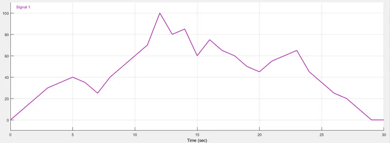
The Sample Drive cycle given

time	0	1	2	3	4	5	6	7	8	9	10	11	12	13	14	15	16	17	18	19	20	21	22	23	24	25	26	27	28	29
flow_rate	0	10	20	30	35	40	35	25	40	50	60	70	100	80	85	60	75	65	60	50	45	55	60	65	45	35	25	20	10	0

This data is imported into a signal builder block and the ramp signal block is replaced with the signal builder block.

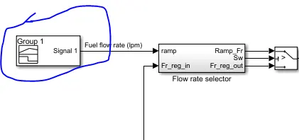
The signal builder input is given below.

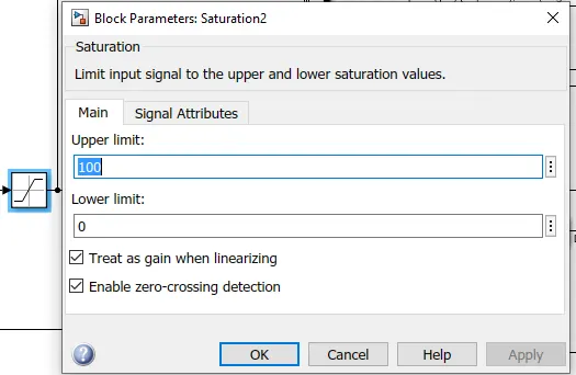
Step 3: Change the upper limit value for flow rate.

The default value given in the block is 85 which is the upper limit value for the ramp signal. The maximum speed value attained during the drive cycle can be given as the upper limit value here.

Step 4: Model the fuel stack

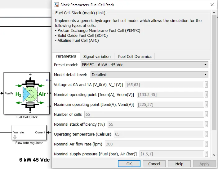
Open the fuel cell stack. We can change the PRESET model of the fuel cell from the drop-down menu. Keeping the type of cell as default because it is the standard type of fuel cell used for EV vehicles. We can give any options from the drop-down menu. But we must make sure our load (driving cycle) and the power rating of the fuel cell are compatible.

Step 5: Run the Simulation

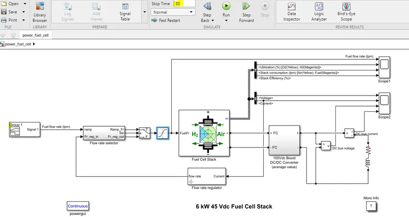
Change the simulation time as per the drive cycle.

OUTPUTS

Scope 1

1.Fuel Flow Rate(lpm)

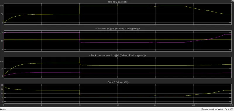
The fuel flow rate increases from 0 to 50lpm in 5seconds. Then it remains 50lpm for the next 5 seconds. At 10seconds the flow rate suddenly rises to 100 and remains constant until 23.75 seconds with a slight variation at 20th second. Then flow rate reduces to 50lpm gradually until 29th second then constant.

2.Utilization(%)-Both Hydrogen and Oxygen

The Hydrogen level is 100% till 10sec and it reduces to 40% between 10sec and 23.5sec. Then we can observe a gradual increase to 88%.

Oxygen level remains at 59.3%

3.Stack Consumption(lpm)

The fuel consumption increases to 50lpm from 0 to 10sec. At 10th second there is a sudden decrease to 40lpm and the consumption is nearly constant from here on.

The consumption of air increases to 178lpm from 0 to 10sec. At 10th second there is a sudden decrease to 145lpm and the consumption is nearly constant from here on.

4.Stack Efficiency(%)

Stack Efficiency decreases from 75% to 55% between 0 to 10sec. At 10th second it suddenly decreases to 27.5% and remains constant till 23.5sec. Then increases to 55% gradually.

Scope 2

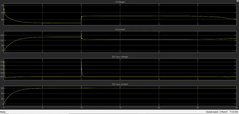
1.Voltage

Voltage decreases from 65V to 45V between 0 to 10sec. Then increases to 55V and remains constant till 23.5sec. Then the voltage decreases to 52V slowly.

2.Current

Current increases from 0 to 135V between 0 to 10sec. Then decreases to 110V and remains constant till 23.5sec. Then the voltage increases to 120V slowly.

3.DC Bus Voltage

This voltage is 100V constant at most of the time expect a peak voltage of 120V at 0sec and 10sec.

4.DC Bus Current

This current increases to 60V at 0 to 5sec. Then remains constant throughout the simulation.

CONCLUSION

A MATLAB model of a fuel cell-powered electric vehicle is simulated.

The results are plotted and analyzed.

*[Simulation File Attached]