Fuel Cell Powered Vehicle Model
Aim:
To make a MATLAB model of fuel powered electric vehicle and comment on the results.
Theory:
A fuel cell is an electrochemical device that generates electricity by consuming a fuel. A fuel cell is one of the various energy storage options apart from batteries and capacitors which are used for an electric vehicle application. Fuel cells are technically not energy storage devices since they do not contain energy that is stored in them like batteries and capacitors do. Instead, fuel cells will undergo a dynamic chemical reaction that will generate the electricity required for propulsive power. The term dynamic means that a continuous supply of fuel and oxygen is required to sustain the chemical reaction. As such, a fuel cell can continue generating electricity for as long as there is a supply of fuel and oxygen provided to it. There are various different types of fuel cells, but they all require the same basic components which are listed below:
Anode:
This is the positively charged electrode, where the fuel is supplied.
Cathode:
This is the negatively charged electrode where oxygen, from the air, is supplied.
Electrolyte:
This is a medium found between the anode and cathode that is permeable to ions but not to electrons. This means that it will allow ions to flow through them, but not electrons.
Anode Catalyst:
This is often fine platinum powder and it helps to catalyse the oxidation of hydrogen gas to hydrogen ions.
Cathode Catalyst:
This is often nickel and helps to catalyse the reduction of oxygen gas to produce the waste products e.g. water.
Gas Diffusion Layers:
These layers help to resist oxidization.
Exhaust:
This is a port through which the exhaust gases i.e. waste products of the chemical reaction can leave the fuel cell. This exists for the excess hydrogen gas also.
We will also study about the BATTERY-TECHNOLOGY and HEV in general.
Definition:
Proton-exchange membrane fuel cells (PEMFC), also known as polymer electrolyte membrane (PEM) fuel cells, are a type of fuel cell being developed mainly for transport applications, as well as for stationary fuel-cell applications and portable fuel-cell applications. Their distinguishing features include lower temperature/pressure ranges (50 to 100 °C) and a special proton-conducting polymer electrolyte membrane. PEMFCs generate electricity and operate on the opposite principle to PEM electrolysis, which consumes electricity.
Working:
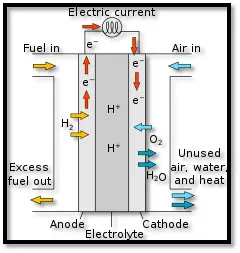
The diagram above shows the basic working of fuel cell. They use a supply of hydrogen gas (H2) as the fuel source and it is supplied to the positively charged anode. A catalyst is used to cause the oxidation of the hydrogen gas. Oxidation is the loss of electrons, and so this process will form positively charged hydrogen ions (H+) which enter the electrolyte. The lost electrons are not permitted to enter the electrolyte and so will travel from the anode to the negatively charged cathode via an external circuit. It is this flow of electrons that produces a direct current electricity supply. The positively charged hydrogen ions will get attracted to the cathode and will move through the electrolyte to get to it. Meanwhile, at the cathode end of the fuel cell, oxygen from the air is supplied to the fuel cell. Another catalyst will cause a chemical reaction at the cathode between the hydrogen ions, electrons and the oxygen gas. This will bring about the reduction of the oxygen gas and will produce water. In addition to electricity and water, fuel cells will also produce heat energy and depending on the type of fuel, very small amounts of nitrogen dioxide and other emissions. If there is any excess hydrogen or oxygen left over, it will exit the fuel cell through a port, to be recycled for use again later on. The overall chemical reaction that occurs in a fuel cell is basically the opposite of electrolysis, where instead of producing hydrogen and oxygen gas from water and electricity, we are doing the reverse. The ionic equation for the chemical reaction that occurs is shown below:
Anode: `H_2 -> 2H^+ + 2e^-`
Cathode: `1/2 O^2 + 2H^+ + 2e^-) -> H_2O`
Overall: `H_2 + 1/2 O_2 -> H_2O`
Model:
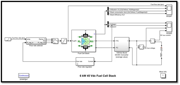
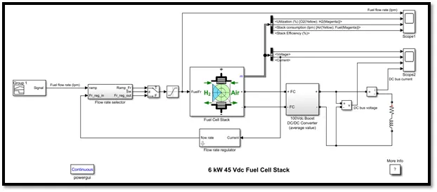
As the name of the model suggests, it has a nominal power of 6 kW and a voltage of 45 Vdc. The model uses a 100 Vdc Boost DC/DC converter which is loaded by an RL element of 6 kW with a time constant of 1 second. A flow rate regulator subsystem is used to control the rate of the fuel supplied to the fuel cell based on the current output of the fuel cell. The flow rate regulator commands the flow rate to the flow rate selector subsystem. The flow rate selector receives an input of a ramp block which has a slope of 10 and is commanded to start after 10 seconds. Based on this ramp input, it will command a fuel flow rate in litres per minute (lpm). This model has 2 scopes to show 2 graphical outputs. The first scope shows the outputs of fuel flow rate in lpm, the oxygen and hydrogen utilization, the stack consumption and the stack efficiency. The second scope shows the voltage and current output of the fuel cell stack. By default, the simulation is made to run for 20 seconds.
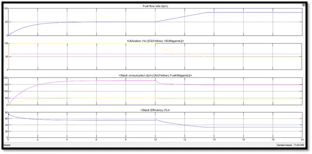
At first, after we run the simulation in its default state for 20 seconds and observed the scopes. The results for Scope 1 are shown below:
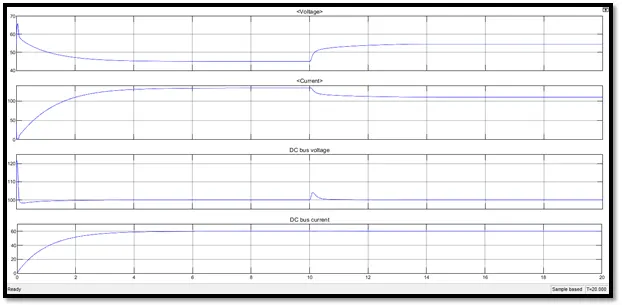
The results of Scope 2 are shown below:
UDDS Drive Cycle
Instead of using the input of the ramp block, I have used the UDDS drive cycle data. Specifically, I used the equivalent current values which correspond to the velocity values against the time. First, I have removed the ramp block, and replaced it with the signal builder block which is shown below:
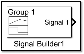
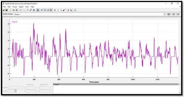
Opening the signal builder block will allow us to modify the signal we wish to input in to the flow rate selector block. I imported the current values of the UDDS drive cycle in to the signal builder block and the signal is shown below:
After this, I decided to run the model with the UDDS current signal for a duration of 200 seconds instead of the full 1369 second duration of the drive cycle. The model with the signal builder block added is shown below:
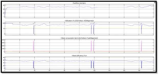
Scope 1 Results:
Fuel Flow Rate
This plot shows how the fuel flow rate of the hydrogen gas varies as the vehicle is being driven according to the UDDS drive cycle. The fuel flow rate of the vehicle fluctuates with time as the drive cycle is run. Initially, the fuel flow rate is 1 lpm at t = 0.037 seconds and this increases to 50 lpm by t = 7.2 seconds where it remains there till t = 20 seconds. This variation in the fuel rate can be explained from the UDDS drive cycle in that the vehicle is at rest till t = 20 seconds. So, the fuel flow rate must have increased in order to prepare the adequate supply of fuel for propulsion after t = 20 seconds. The vehicle must be receiving a standby fuel flow rate of 50 lpm whenever at rest.
After t = 20 seconds, the vehicle speed begins to increase and this is reflected in the fuel flow rate increasing also. At t = 26 seconds the fuel flow rate is 53.5 lpm and at t = 27 seconds, the fuel flow rate decreases to 50.9 lpm in spite of the vehicle speed increasing. This decrease in the fuel flow rate is because after t = 26 seconds, the acceleration of the vehicle decreased. The fuel flow rate again increases to 54.35 lpm at t = 29 seconds because the acceleration of the vehicle increased. At x = 38, the fuel flow rate decreased to 47.6 lpm, which is lower than the starting 50 lpm and this is explained by the vehicle decelerating for the first time in the drive cycle. This occurs once again when the vehicle decelerated at t = 53 seconds causing the fuel flow rate to drop to 48 lpm. At x = 116 seconds, the fuel flow rate reaches a minimum dropping to 45.6 lpm. This corresponds to the greatest value of the deceleration of the vehicle from 13m/s to rest. The vehicle remains at rest t = 125 seconds to t = 163 seconds and this is seen in the fuel flow rate returning to its standby value of 50 lpm. The fluctuations continue once again as per the acceleration of the vehicle.
Fuel Utilization
This plot shows how the hydrogen and oxygen is being used in the fuel cell as the vehicle is being run according to the UDDS drive cycle. We can see that the magenta and turquoise lines represent the utilization of hydrogen and oxygen respectively. The most noticeable observation is that the hydrogen gas utilization is constant throughout the entire drive cycle remaining at 59.3%. This must be because the fuel cell demands that there always be a standby supply of hydrogen available. So if the vehicle is accelerating or decelerating, the fuel flow rate increases or decreases respectively above the standby value of 50 lpm and when the vehicle is at rest, the fuel flow rate is exactly 50 lpm. However, the O2 utilization fluctuates throughout the drive cycle. Initially, the O2 utilization was at 99.47% and remains there till t = 10 seconds before rapidly falling to 88.4% at t = 12 seconds where it remains till t = 20 seconds. During this period, the vehicle was at rest and so the O2 utilization decreased to its standby value of 88.4% because while at rest, 100% utilization is not required.
After t = 20 seconds, the O2 utilization decreases to 80.7% at t = 26 seconds but increases back to 85.8% at t = 27 seconds. This decrease then increase in the O2 utilization is due to the decrease in the acceleration of the vehicle during those times. When the vehicle acceleration increases, the O2 utilization falls and vice versa. This is perhaps because increased acceleration requires more power and this is reflected in the higher fuel flow rate of hydrogen. However, when the vehicle acceleration decreases, the O2 utilization rises and this is because less power and hence less hydrogen is required by the fuel cell. After this, the O2 utilization increases to 99.99% at t = 32 seconds but this is only for an instant as the utilization drops dramatically to 0.01% at t = 38.6 seconds and this corresponds to the vehicle speed decreasing to 6.6 m/s. The same occurs at t = 116 seconds where the vehicle undergoes its greatest deceleration back to rest causing the O2 utilization to decrease from 99.99% to 0.01% within 0.1 seconds. So, we can understand that decelerating beyond a certain value will decrease the O2 utilization to 0.01%. This must be because deceleration requires no power from the fuel cell and so its dependency on oxygen is almost 0%. The vehicle returns to rest between t = 125 seconds and t = 162 seconds causing the O2 utilization to return to its standby value of 88.4%.
Stack Consumption
This plot shows how the amount of hydrogen and oxygen available is consumed from the fuel cell stack. The consumption of O2 is initially at 27.46 lpm at t = 0.001 seconds and fluctuates to 56.2 lpm at t = 0.005 seconds. The O2 consumption decreases back to 4.2 lpm at t = 0.08 seconds and then begins to increase rapidly with the plot having a shape similar to a quadratic curve. The O2 consumption levels off and settles at 178 lpm at t = 10 seconds after which the consumption reduces to 157 lpm and remains there till t = 20 seconds. After t = 30 seconds, there is a small increase in the O2 consumption before shooting up rapidly at t = 38 seconds reaching a maximum value of 3726 lpm at t = 38.26 seconds. This is only maintained for an instant before falling to 0.04 lpm at t = 38.6 seconds before shooting up again and levelling off at 155 lpm where it is stable again. This rapid decrease in the O2 consumption is due to the rapid deceleration of the vehicle during those periods before accelerating again. The O2 consumption shoots up again rapidly reaching maximum values at t = 116 and 119 seconds. This shooting up of the O2 consumption occurs whenever the vehicle has a high deceleration and this is observed in the UDDS drive cycle. However, when the vehicle accelerates or is at rest, it has a stable value of approximately 155 lpm. This may be due to the fact that acceleration demands more hydrogen in the fuel cell and so we do not see any increased O2 consumption during those periods.
The consumption of hydrogen is similar to the shape of the plot for the O2 consumption. Initially, the hydrogen consumption is 0 at t = 0 seconds, and this is because the vehicle is initially t rest and so did not consume any hydrogen fuel. The consumption then increases to approximately 49 lpm at t = 5 seconds where it remains stable till t = 10 seconds. From t = 10 seconds till t = 35 seconds, the hydrogen consumption decreases to 44 lpm and remains there. However, at t = 38.26 seconds, the hydrogen consumption increases slightly and this coincides with the rapid increase of the O2 consumption to reach its maximum value. But the hydrogen consumption immediately falls to a minimum value of 0.0048 lpm at t = 38.26 seconds and this is coincides with the minimum O2 consumption as well. By t = 40 seconds, the hydrogen consumption shoots back up again and remains stable at approximately 43 lpm. The hydrogen consumption falls to its minimum again at t = 116 and 119 seconds and this coincides with the minimum O2 consumption. The sudden decreases in the hydrogen consumption is due to the deceleration of the vehicle and when the vehicle is accelerating or at rest, the hydrogen consumption is quite stable.
Stack Efficiency
This plot shows the efficiency of the fuel cell stack with the drive cycle. Initially, the stack efficiency is 0% at t = 0 seconds and rises rapidly to 75.78% at t = 0.07 seconds. But this is maintained only for an instant before decreasing and levelling off at 55% at t = 10 seconds. After t = 10 seconds, there is a small spike in the efficiency to 56.55% before returning to 55% and it remains there till t = 20 seconds. After t = 20 seconds, the vehicle begins to accelerate and this causes the stack efficiency to decrease 51.5% at t = 26 seconds. The stack efficiency increases to 54% t = 27 seconds and then drops again 50.8% at t = 28 seconds. The efficiency drops during this time due to the decrease in the acceleration during this period. At t = 38 seconds, the stack efficiency falls to 0% and this corresponds to the rapid deceleration of the vehicle. So, a deceleration beyond a certain value will cause the stack efficiency to drop dramatically to 0%. However, the 0% efficiency is maintained for an instant and shoots up back to 54% at t = 54 seconds and fluctuates again between 50 - 57%. The stack efficiency decreases when the vehicle accelerates and when rapidly braking. The stack efficiency drops to 0% on two more instances at t = 116 seconds and t = 119 seconds and this corresponds to the rapid deceleration of the vehicle from 13 m/s to rest. When the vehicle is at rest between t = 125 and t = 162 seconds, the stack efficiency remains stable at 55% which was observed in the first 20 seconds as well.
Scope 2 Results:
Voltage
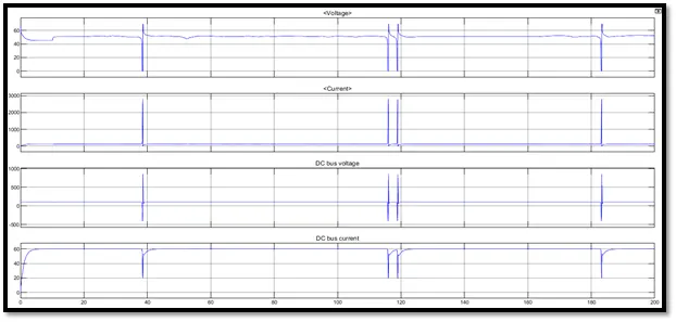
The voltage plot shows how the voltage in the fuel cell varies with time for the UDDS drive cycle. We can see that in general the voltage seems to fluctuate between 52V and 48V for the majority of the time but also shows sudden instantaneous spikes where the voltage drops as low as 0V and as high as 69.5V. Initially, the voltage is at approximately 69.52V at t = 0 seconds and this decreases rapidly to 45V at t = 10 seconds before increasing again to 50.8V and remaining there till t = 20 seconds. From the UDDS drive cycle, we know that the vehicle is at rest for the first 20 seconds, and so the standby voltage of the fuel cell stack must 50.8V corresponding to the vehicle being at rest. After this, the vehicle accelerates and this is reflected in the increase in the voltage to 52V at t = 26 seconds. However, the voltage decreases again but very slightly to 51V at t = 27 seconds before increasing again after. This fluctuation in voltage is explained by the change in the motion of the vehicle. At first, its acceleration was constant, but then it reduced at t = 26 seconds causing the decrease in voltage. But after this, the vehicle accelerates again bringing the voltage up once more. At t = 36.7 seconds, the voltage is at 50.6V and this undergoes a dramatic decrease to 0 at t = 38.4 seconds. Immediately after, the voltage shoots up to 69.6V at t = 38.6 seconds. This sudden rapid decrease and increase in the voltage corresponds to the vehicle decelerating for the first time in the drive cycle to 6.6m/s before accelerating again. The voltage again spikes like this at t = 114 seconds and this corresponds to the vehicle decelerating once again but this time back to rest. When the vehicle is at rest at t = 122 seconds to t = 162 seconds, the voltage remains constant at 50.7V and this was seen in the first 20 seconds of the plot.
Current
The current plot shows how the current in the fuel cell stack varies with time for the UDDS drive cycle. We can see that for the majority of the drive cycle, the current is at approximately 117A and at few instances, there are current spikes. Initially, the current is at 0A at t = 0 seconds. Immediately after the current undergoes a sharp spike to 42.25A at t = 0.005 seconds before a sharp decrease to 2.6A at t = 0.07 seconds. From here, the current increases rapidly to 133.3A at t = 6 seconds and remains there till t = 10 seconds. After t = 10 seconds, the current decreases rapidly before levelling off at 118A at t = 12 seconds where it remains till t = 20 seconds. Since we know that the vehicle is at rest till this point, we can assume that the standby current of the fuel cell is approximately 118A when the vehicle is at rest. After t = 20 seconds, the vehicle begins to accelerate and this causes the current to decrease very slowly to 115A at t = 26 seconds before increasing to 117A at t = 27 seconds. The decrease in the current occurs when the vehicle begins to accelerate whereas the slight increase in the current is due to the reduction in acceleration of the vehicle. These fluctuations continue as the vehicle's acceleration varies. At t = 38 seconds, the vehicle undergoes its first deceleration from 10m/s to 6.6m/s and this causes the current to undergo its first massive spike causing the current to increase from 125A to 2796A within 0.5 seconds. Immediately after, the current instantaneously drops to -0.06A by t = 38.6 seconds before shooting up to a more stable level of 116A at t = 42 seconds. These massive spikes are seen again at t = 116 and t = 119 seconds which correspond to the rapid deceleration of the vehicle from 14m/s to rest. When the vehicle is at rest between t = 125 and t = 162 seconds, the current remains constant at its stable value of 118.2A.
DC Bus Voltage
The DC bus voltage plot shows how the voltage varies in the boost converter with time. In general, the DC bus voltage remains constant at 100V for the majority of the drive cycle and this is due to the fact that the boost converter is supposed to output a voltage of 100V. There are a few spikes in the voltage across different wherein the voltage suddenly increases and then decreases. Initially, the DC bus voltage is at 100V and suddenly shoots up to 121V at t = 0.012 seconds and falls to 98.27V at t = 0.2 seconds before levelling off at 100V at t = 5 seconds where it remains till t = 10 seconds. At t = 10.2 seconds, there is a small instantaneous spike in the voltage to 102.8V before returning to the standby 100V value. The DC bus voltage remains there until t = 38 seconds, where the first major spike occurs. The voltage decreases dramatically to -412.4V at t = 38.46V before immediately increasing to the peak value at 852V at t = 38.6 seconds. Once again, the DC bus voltage decreases back to 58.46V at t = 38.72 seconds. Within 0.01 seconds, the DC bus voltage again increases to 58.99V and then continues to increase back to the standby level of 100V at t = 42 seconds. This sudden spike and fall in the DC bus voltage occurs due to the deceleration of the vehicle at that time. The DC bus voltage behaves this way again a few more times with the next time occurring at t = 115 seconds when the vehicle decelerates rapidly from 14 m/s to rest. When the vehicle is at rest between t = 125 and 162 seconds, the DC bus voltage remains constant at 100V.
DC Bus Current
The DC bus current plot shows how the current varies in the boost converter with time. In general, the DC bus current remains constant at 60A with various instantaneous fluctuations occurring at different instances. Initially the DC bus current is 0A and as the time elapses, it increases rapidly and levels off at 60A by t = 10 seconds. At t = 10.48 seconds, there is a small spike in the DC bus current to 60.31A before gradually returning to 60A at t = 14.2 seconds where it remains till t = 20 seconds. From here, the DC bus current is more or less constant at 60A with a few small deviations. One such small deviation is at t = 27.1 seconds where the current drops to 59.97A and this occurs due to the decrease in the acceleration of the vehicle. The first of few fluctuations occurs at t = 37 seconds, where the DC bus current rapidly drops from 60A to 19.51A at t = 38.57 seconds. From here the current increases instantaneously to 53.1A at t = 38.72 seconds before again dropping to 51.89A at t = 38.99 seconds and after, returns immediately to 60A at t = 45 seconds. This fluctuation in the DC bus current can be attributed to the deceleration of the vehicle till 6.6m/s at t = 39 seconds before accelerating again. At t = 115 seconds, the vehicle begins its next deceleration from 13m/s to rest by t = 125 seconds, and this is seen as the second set of fluctuations in the DC bus current similar to before. This fluctuation only occurs when the vehicle decelerates beyond a certain value because when the vehicle is at rest e.g. between t = 125 and 162 seconds, the DC bus current remains at its constant value of 60A. These fluctuations continue on whenever the vehicle undergoes a significant deceleration.
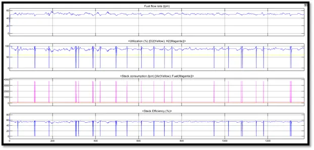
The image below shows the Scope 1 results for the full duration of the UDDS drive cycle.
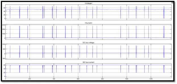
The image below shows the Scope 2 results for the full duration of the UDDS drive cycle.
Conclusion:
In conclusion, the 6kW 45Vdc fuel cell stack model has been simulated with the corresponding current values of the UDDS drive cycle and the observations of the fuel flow rate, utilization of hydrogen and oxygen, stack consumption and stack efficiency have been plotted against the time in the first scope, and the observations of the voltage, current, DC bus voltage and DC bus current have been plotted against the time in the second scope. The results have been analysed and they have been explained in detail comparing the data with the UDDS drive cycle data.