Genetic Algorithm

General syntax of ‘ga’:

[x,fval] = ga (fitnessfcn, nvars, A, b, Aeq, beq, lb, ub, noncoln, options)

‘x’ inputs the return values.

‘fval’ returns the value of the fitness function.

‘fitnessfcn’ is the function which we desire to minimize.

‘nvars’ are the number of variables associated with the function.

‘A, b, Aeq, beq’ is used when the inequalities are used.

‘lb, ub’ is used to set the lower and upper bounds of search space.

‘noncoln’ sets the non-linear constraint

‘intcoln’ sets the integer constraint

‘options’ is used to change the parameters of the ga.

The given function is as follows,

`f(x,y) = f underset(1,x)` `f underset(2,x)` `f underset(1,y)` `f underset(2,y)`

`f underset(1,x)``= [sin(5.1pix + 0.5)]^6`

`f underset(1,y)``= [sin(5.1piy + 0.5)]^6`

`f underset(2,x)``= exp [-4log(2) (x-0.0667)^2 / 0.64]`

`f underset(2,y)``= exp [-4log(2) (y-0.0667)^2 / 0.64]`

where x and y are the two variables.

Code:

Function Code:

function [f] = stalagmite(input_value)
f_1_x = (sin(5.1*pi*input_value(1) + 0.5))^6;
f_1_y = (sin(5.1*pi*input_value(2) + 0.5))^6;
f_2_x = exp(-4*ln(2)*(((input_value(1) - 0.0667)^2)/(0.64)));
f_2_y = exp(-4*ln(2)*(((input_value(2) - 0.0667)^2)/(0.64)));
f = -(f_1_x*f_1_y*f_2_x*f_2_y)
end

Parent Code:

clear all
close all
clc

%Defining our search space
x = linspace(0,0.6,150);
y = linspace(0,0.6,150);
num_cases = 50

%Creating a 2Dimensional mesh
[xx yy] = meshgrid(x,y);

%Evaluating the stalagmite function
for i = 1:length(xx)
    for j = 1:length(yy)
        input_value(1)=xx(i,j);
        input_value(2)=yy(i,j);
        f(i,j) = stalagmite(input_value);
    end
end

%Study 1 - Statistical behavior

tic

for i = 1:num_cases
    [inputs, fopt(i)] = ga(@stalagmite,2);
    xopt(i) = inputs(1);
    yopt(i) = inputs(2);
end

study1_time = toc

figure(1)
subplot(2,1,1)
hold on 
surf(xx,yy,f)
shading interp
plot3(xopt, yopt, fopt,'marker','o','markersize',5,'markerfacecolor','r' )
title('Unbounded inputs')
subplot(2,1,2)
plot(fopt)
xlabel('Iterations')
ylabel('Function maximum')

%Study 2 - Statistical behavior - with lower and upper bounds

tic

for i = 1:num_cases
    [inputs, fopt(i)] = ga(@stalagmite,2,[],[],[],[],[0;0],[1;1]);
    xopt(i) = inputs(1);
    yopt(i) = inputs(2);
end

study2_time = toc

figure(2)
subplot(2,1,1)
hold on
surf(xx,yy,f)
shading interp
plot3(xopt, yopt, fopt,'marker','o','markersize',5,'markerfacecolor','r' )
title('Bounded inputs')
subplot(2,1,2)
plot(fopt)
xlabel('Iterations')
ylabel('Function maximum')

%Study 3 - Increasing GA iterations

options = optimoptions('ga');
options = optimoptions(options,'PopulationSize',200)

tic

for i = 1:num_cases
    [inputs, fopt(i)] = ga(@stalagmite,2,[],[],[],[],[0;0],[1;1],[],[],options);
    xopt(i) = inputs(1);
    yopt(i) = inputs(2);
end

study3_time = toc

figure(3)
subplot(2,1,1)
hold on
surf(xx,yy,f)
shading interp
plot3(xopt, yopt, fopt,'marker','o','markersize',5,'markerfacecolor','r' )
title('Bounded inputs with modified population size')
subplot(2,1,2)
plot(fopt)
xlabel('Iterations')
ylabel('Function maximum')

Explanation of Code:

Function Code:

The stalagmite function takes a row vector named 'input_value' as an input.

The equations are defined in the function and is finally multiplied by '-1' to invert the function about x-axis. This is done since 'ga' algorithm always minimises the fitness function, but we need maximisation as the ouput.

Parent Code:

'linspace' command is used to assign a total of 150 values between the range 0 to 0.6 for the values of x and y.

'meshgrid' command is used to convert the values of x and y into 2d mesh.

Study 1:

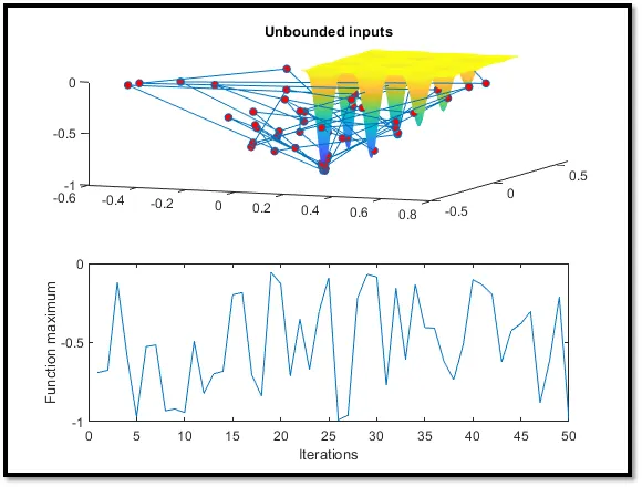
In general the inbuild solver of genetic alrgorithm calculates 50 iterations and the output is assigned in the array inputs and fopt(i).

xopt is assigned the 1st column of values and yopt is assigned the 2nd column of values.

'subplot' command is used to create two plots attached one after the other.

'surfc' command is used to create 3d plot.

'shading interp' command is used to remove the grids from the command and to display surface texture of 3d plot.

Study 2:

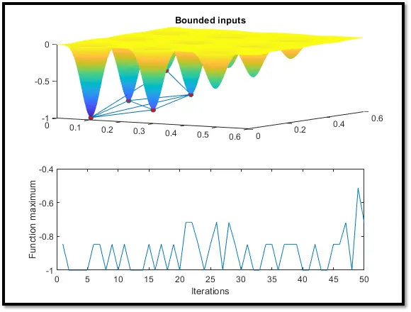
ga(@stalagmite, 2, [], [], [], [], [0;0], [1;1]);

'ga' is used to call the genetic algorithm solver.

'@stalagmite' is used to call our function.

'2' is used to define the number of variables i.e., x and y in our program.

first '[], []' means that there are no linear inequalities existing between x and y.

second '[], []' means that there are no linear inequalities existing between xeqn and yeqn.

'[0,0]' represents the lower boundary conditions of x and y.

'[1,1]' represents the upper boundary conditions of x and y.

Study 3:

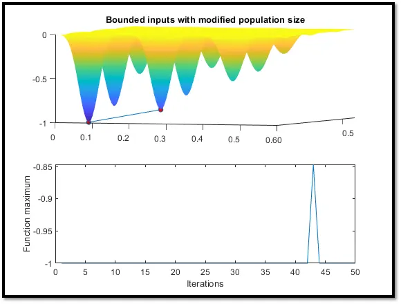
In the last study we are going to change the inbulit parameter of population in ga solver to 300 by using the optimoptions command as follows:

options = optimoptions (optimoptions, 'PopulationSize', 200)

We will also change the syntax of ga compared to the last study as follows:

ga(@stalagmite, 2, [], [], [], [], [0;0], [1;1], [], [], options);

'ga' is used to call the genetic algorithm solver.

'@stalagmite' is used to call our function.

'2' is used to define the number of variables i.e., x and y in our program.

first '[], []' means that there are no linear inequalities existing between x and y.

second '[], []' means that there are no linear inequalities existing between xeqn and yeqn.

'[0,0]' represents the lower boundary conditions of x and y.

'[1,1]' represents the upper boundary conditions of x and y.

third '[], []' means that there are no linear constraints.

Output:

Study 1:

Study 2:

Study 3:

Errors faced while programming:

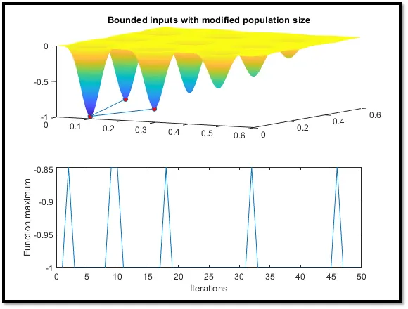
Since the population is 170 we are getting variation.

Steps taken to overcome the error:

The population is increased to 200 to avoid this error and so we get the results as follows.

Conclusion:

The program to explain the stalagmite function and genectic algorithm for the given function has been discussed in this project. The global maxima of the given function is also found out and the graphs are plotted for all the 3 studies for function maximum and number of iterations.

References:

1. https://www.tutorialspoint.com/genetic_algorithms/genetic_algorithms_quick_guide.htm
2. https://in.mathworks.com/help/gads/ga.html#mw_d9f21ac7-dfb6-4e81-bbdc-c1cb5533af18
3. https://towardsdatascience.com/introduction-to-genetic-algorithms-including-example-code-e396e98d8bf3