Solving second order ODEs
Aim : To solve the second order Ordinary Differential Equation using the example of simple pendulum that describes the position of the bob with respect to time using MATLAB. The program is computed to represent the motion of the pendulum with damping and also to simulate the motion of the pendulum.
Governing Equations : In this program we are going to solve the ODE which represents the equation of motion of a simple pendulum with damping,
`(d^2theta)/dt^2 + b/m (d theta)/dt + g/L sin theta = 0`
where,
g = gravity in `m/s^2`,
L = length of the pendulum in m,
m = mass of the ball in kg,
b = damping coefficient
In order to solve a higher order ODE, you have to break it down into a set of first order ODE.
First order ODE means `(d theta)/dt` and second order ODE means `(d^2theta)/dt^2`
Here we assume, `theta =theta_1`
So,
`(d theta)/dt = (d theta_1)/dt = theta_2` ----- (1)
`(d^2theta)/dt^2 = (d^2theta_1)/dt^2 = d/dt ((d theta_1)/dt) = (d theta_2)/dt` ----- (2)
We have the equation,
`(d^2theta_1)/dt^2 + b/m (d theta_1)/dt + g/L sin theta = 0`
Substituting equations (1) and (2) in the above equation, we get
`(d theta_2)/dt + b/m theta_2 + g/L sin theta_1 = 0`
Hence,
`(d theta_2)/dt = -b/m (d theta_2)/dt - g/L sin theta_1`
We know,
`(d theta_1)/dt = theta_2`
So,
`d/dt ((theta_1), (theta_2)) = ((theta_2), (-b/m theta_2 -g/L sin theta_1))`
Objective of the project :
The main objective of the project is to solve a second order ODE by using the equation of motion of a simple pendulum. Initially, we are going to break down the second order ODE into first order ODE. Now, we will provide a separate function, which we call into the main program.
In order to solve the ODE we are going to use the ode45 solver whose syntax is
[t,y] = ode45(odefun,tspan,y0,options)
where tspan = [t0 tf], integrates the system of differential equations from t0 to tf with the initial conditions y0. Each row in the solution array y corresponds to a value returned in column vector t.
Code :
%ODE funtion code
function [dtheta_dt] = ode_func(t,theta,b,g,l,m)
theta1 = theta(1)
theta2 = theta(2)
dtheta1_dt = theta2;
dtheta2_dt = -(b/m)*theta2-(g/l)*sin(theta1);
dtheta_dt = [dtheta1_dt;dtheta2_dt];
end
%Solving second order ODE
clear all
close all
clc
%Inputs
b = 0.05;
g = 9.81;
l = 1;
m = 0.1;
%Initial condition
theta_0 = [0;3];
%Time points
t_span = linspace (0,20,500);
%Solve ODE
[t, results] = ode45(@(t,theta)ode_func(t,theta,b,g,l,m), t_span,theta_0);
%Plotting the graph
figure (1);
plot (t, results(:,1))
hold on
plot (t, results(:,2))
xlabel('Time')
ylabel('Plot')
theta_1 = results(:,1);
ct = 1;
for i = 1:length(theta_1)
THETA_1 = theta_1(i);
%Motion of pendulum
x0 = 0;
y0 = 0;
x1 = l*sin(THETA_1);
y1 = -l*cos(THETA_1);
%Plotting the motion
figure(2);
plot([x0 x1],[y0,y1],'color','b');
hold on
plot(x1,y1,'o','markersize',20,'color','r','MarkerFaceColor','r')
hold off
axis([-1.5 1.5 -1.5 0.5])
pause(0.01)
M(ct) = getframe(gcf);
ct = ct+1;
end
movie(M)
videofile = VideoWriter('pendulum.avi','uncompressed avi');
open(videofile)
writeVideo(videofile,M)
close(videofile)Explanation of the Code :
According to the results from our governing equations we have the values as follows,
`d/dt ((theta_1), (theta_2)) = ((theta_2), (-b/m theta_2 -g/L sin theta_1))`
Now we are going to implement this equation as the calling function for our main code which is shown as the first programming code.
Next we are going to proceed with our main code by inputting the values of damping co-efficient, gravity, length of the pendulum and mass as provided in the problem statement.
We are solving a second order ODE which has one for velocity and displacement. So, we are alloting the values of initial displacement and initial velocity for the term theta_0
For the time points, the time array is used to intergrate the ODE for the input values for the time span 0-20 secs.
While solving the ODE we use ode45 for the function of @(t,theta) and the input parameters ode_func(t,theta,b,g,l,m) is a separate funtion which is called from the first programming code. t_span and theta_0 are the options which are used in the ode45 solver where t_span is the time array which teels us how far the intergration needs to be done and theta_0 is the starting of the time with the initial conditions.
The plotting results will have a colmun vector and it will have two columns. The first column will have displacement and the second column will have velocity.
Now, we will get the plot for damping effect on a simple pendulum with respect to displacement and velocity for the time span mentioned.
In order the animate the motion of the simple pendulum we are going to use the for loop for the time span mentioned in the problem statement.
'ct' command i.e., the counter command is assumed a value of 1 initally to store the whole execution of the upcoming 'for loop' command.
'length(theta1)' command represents the number of values in theta1.
We are going to assign the initial position of the pendulum as x0 and y0 and then we are going to formulate x1 and y1 for the respective theta values which will vary according to the displacement and velocity and the movement of the pendulum will be simulated till the for loop terminates.
In order to represent the bob of the pendulum we are going to use the markersize command and we are going to plot the string attached to the bob.
'axis' command is used to give the x and y limits for the plot with respect to which the plotting of the robotic arm will be represented.
'plot' command is used to visualize all the plots in a single picture video or in a single GIF with all the different positions of the simple pendulum.
'getframe' command is used to get individual frames and save it in a array of 'M(ct)'.
'movie(M)' command generates a movie of the values stored in 'M'.
'videofile' command is used to save it with the file name pendulum.
'writeVideo' command is used to write into the video file with the frames of M.
Errors faced while programming :
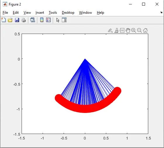
Error 1 : Simulation of the pendulum was not clear.
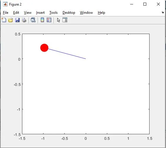
Error 2 : Motion of the pendulum was not properly visible.
Steps taken to overcome the errors :
Step 1 : 'hold off' command was used to set the hold state to off so that new plots added to the axes clear existing plots and reset all axes properties.
Step 2 : x1 and y1 values were found out to make sure the motion of the pendulum is visible inside the aixs area.
Screenshots of the error :
Error 1 :
Error 2 :
Conclusion :
Output video link :
Graph plot :
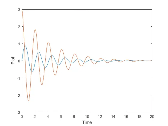
The output video link shows the motion of the simple pendulum and the graph plot represents the damping effect on the pendulum with respect to the given parameters.