Week 6 - Data analysis

Aim:

To develop a Python script to establish a versatile and automated tool for data analysis that emphasizes visualization, compatability and performance calculations for an engine data.

Objective:

Data visualizer

• Your script should take column numbers as the input and plot the respective columns as separate images
• Each file should be saved by the name of the column
• The plot labels should be extracted from the file. If, I request for a plot between column 1 (crank angle) and column 8(volume), then the label information should automatically be extracted and must appear as labels in the plots. THIS SHOULD NOT BE DONE MANUALLY

Compatability check

• You code should exit gracefully, if a non-compatible file is provided as an input. It should say something like "File not recognized. Please provide a valid CONVERGE output file"

Basic performance calculation

• Calculate the area under the P-V diagram. P is in column 2 and V is in column 8.
• Calculate the power output of this engine. Assume that RPM is 1500
• This engine consumed 20 micro grams of fuel (per 1 stroke cycle). Calculate its specific fuel consumption.

Problem Statement:

Data Analysis

Analysis involves breaking down a whole into its individual components for thorough assessment. The process of data analysis involves acquiring raw data and transforming it into information that aids users in decision-making. Data is collected and scrutinized to address queries and test hypotheses.

Utilizing data analysis contributes to enhancing the scientific nature of decision-making and improving operational efficiency for businesses. Data analysis involves the systematic examination, cleansing, transformation, and modeling of data, with the objective of uncovering valuable insights, guiding conclusions, and facilitating informed choices. Data analysis encompasses a range of methods and strategies, with various techniques falling under different names. It finds application in diverse sectors such as business, science, and social sciences.

Statistician John Tukey, defined data analysis in 1961, as:

"Procedures for analyzing data, techniques for interpreting the results of such procedures, ways of planning the gathering of data to make its analysis easier, more precise, or more accurate, and all the machinery and results of (mathematical) statistics which apply to analyzing data."

The classification of data analysis includes four main types:

• Descriptive Analysis

This helps with the 'what' statement. example : What is happened to your business? This is done with live data helps in effective visualisation. This analysis the past data.

TOOLS AND TECHNIQUIES USED : metrics and statistics

• Diagnostic Analysis

This comes up with the 'why' statement. example : Why this is happened? This helps to understand the root of your problem. This is also analysis the past data.

TOOLS AND TECHNIQUIES USED : PCA and regression analysis

• Predictive Analysis

This comes up with the 'if' statement. example: What will happenend if this occurs? This helps to understand the prediction of the future. History helps in predicting the future.

TOOLS AND TECHNIQUIES USED : machine learning algorithms

• Prescriptive Analysis

It help in the 'recommendataion" statement. example : What should i do if this happen, What are the possible recommendation. This is also helps in understanding the future.

TOOLS AND TECHNIQUIES USED : neutral network, recommeder system.

The provided data file contains diverse engine parameters, and the task involves computing the following parameters:

1. The work done by the engine, which is derived by determining the area under the PV diagram.
2. The engine power output, which is determined as follows:

Where,

𝑾𝒐𝒖𝒕 is the work output of the engine

𝑹𝑷𝑴 is the engine speed (rev/min)

𝒏 is the number of engine cylinders

3. Specific fuel consumption (sfc)

Program:

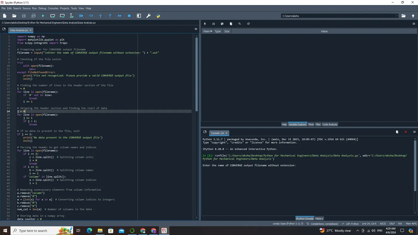
import sys
import numpy as np
import matplotlib.pyplot as plt
from scipy.integrate import trapz

# Prompting user for CONVERGE output filename
filename = input("\nEnter the name of CONVERGE output filename without extension: ") + ".out"

# Checking if the file exists
try:
    with open(filename):
        pass
except FileNotFoundError:
    print('File not recognized. Please provide a valid CONVERGE output file')
    sys.exit()

# Finding the number of lines in the header section of the file
i = 0
for line in open(filename):
    if '#' not in line:
        break
    i += 1

# Skipping the header section and finding the start of data
j = 0
for line in open(filename):
    j += 1
    if j > i:
        break

# If no data is present in the file, exit
if j == i:
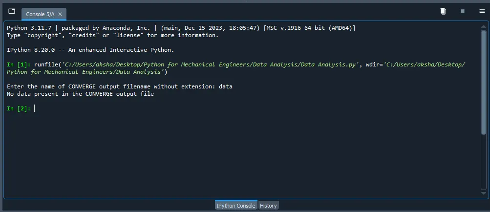
    print('No data present in the CONVERGE output file')
    sys.exit()

# Parsing the header to get column names and indices
for line in open(filename):
    if i == 2:
        c = line.split()  # Splitting column units
        i = 0
        break
    if i == 1:
        b = line.split()  # Splitting column names
        i += 1
    if 'column' in line.split():
        a = line.split()  # Splitting column indices
        i = 1

# Removing unnecessary elements from column information
a.remove("column")
a.remove("#")
a = [int(x) for x in a]  # Converting column indices to integers
b.remove("#")
c.remove("#")
num_col = len(a)  # Number of columns in the data

# Storing data in a numpy array
data_counter = 0
data = np.arange(0, num_col)

for line in open(filename):
    if '#' not in line:
        d = line.split()  # Splitting data points
        d = np.array(d, dtype=np.float32)  # Converting data points to float32
        data = np.vstack([data, d])  # Stacking data points
        data_counter += 1

data = np.delete(data, 0, 0)  # Deleting the initial placeholder row

# Displaying available variables for plotting
print('\nType -')
for i in a:
    print('{} for {}'.format(i, b[i - 1]))  # Displaying column indices and names

print('')
x = input("Do you want a plot between any two variables? (y/n): ")

# Interactive plotting loop
while x.lower() == 'y':
    cn1 = int(input("Enter the column number of the variable along X-axis (Refer input map above): "))
    cn2 = int(input("Enter the column number of the variable along Y-axis (Refer input map above): "))
    plt.figure()
    plt.plot(data[:, cn1 - 1], data[:, cn2 - 1])  # Plotting selected data
    plt.xlabel('{} {}'.format(b[cn1 - 1], c[cn1 - 1]))  # Labeling X-axis
    plt.ylabel('{} {}'.format(b[cn2 - 1], c[cn2 - 1]))  # Labeling Y-axis
    plt.title('{} {} vs {} {}'.format(b[cn2 - 1], c[cn2 - 1], b[cn1 - 1], c[cn1 - 1]))  # Setting plot title
    z = input("Do you want to save the plot? (y/n): ")
    if z.lower() == 'y':
        plt.savefig("{}-{}.png".format(b[cn2 - 1], b[cn1 - 1]))  # Saving plot
        plt.show()  # Displaying plot
        print('')
        x = input("\nDo you want to plot any other two variables? (y/n): ")  # Prompting for more plots
    else:
        plt.show()  # Displaying plot
        print('')
        break  # Exit the loop if the plot is not saved
        
# Engine performance analysis
print('\nPERFORMANCE OF THE ENGINE')

# Finding columns for pressure and volume
b1 = [i.lower() for i in b]  # Converting column names to lowercase for case-insensitive search
pressure_column = b1.index('pressure')  # Finding pressure column index
volume_column = b1.index('volume')  # Finding volume column index

# Extracting pressure and volume data
pressure = data[:, pressure_column]  # Extracting pressure data
volume = data[:, volume_column]  # Extracting volume data

# Calculating work done per cycle (Area under P-V curve)
A = trapz(pressure, volume) * 1e6  # Calculating area under the curve

# Taking input from user for RPM and fuel consumption
rpm = float(input('\nEnter the rpm of the engine at which data was collected: '))
fuel_consumed_per_cycle = float(input('Enter the value of the fuel consumed per cycle (in micrograms): '))

# Calculating power output and specific fuel consumption
speed = (rpm / 60) / 2  # Converting rpm to cycles per second
P = A * speed  # Calculating power output
f = (fuel_consumed_per_cycle * rpm * 3600) / 1e9  # Converting micrograms to kilograms and adjusting for time
sfc = (f * 1000) / P  # Converting fuel consumption to kg/kW.hr

# Displaying results
print('\nArea under the P-V curve (Work done per cycle): {} J'.format(A))
print('\nPower output at {} rpm: {} kW'.format(rpm, P/1000))
print('\nSpecific fuel consumption: {} Kg/KW.hr'.format(sfc))

#Plotting area under PV
plt.plot(volume, pressure, color='blue', label='PV curve')
plt.fill_between(volume, pressure, color='lightblue', label='Area under curve')
plt.xlabel("Volume")
plt.ylabel("Pressure")
plt.legend()
plt.title("P-V Diagram and Area under Curve")
plt.savefig("area_under_PV_curve.png")
plt.show()

Explanation:

This Python script is to establish a versatile and automated tool for data analysis that emphasizes visualization, compatability and performance calculations for an engine data. Let's break down the code step by step:

Importing Variables

import sys
import numpy as np
import matplotlib.pyplot as plt
from scipy.integrate import trapz

• sys: for system-specific parameters and functions.
• numpy (as np): for numerical computing.
• matplotlib.pyplot (as plt): for plotting graphs.
• trapz from scipy.integrate: for numerical integration using the trapezoidal rule.

User Input and File Validation

This section handles user interaction to obtain the filename of the CONVERGE output file and ensures its validity.

# Prompting user for CONVERGE output filename
filename = input("\nEnter the name of CONVERGE output filename without extension: ") + ".out"

# Checking if the file exists
try:
    with open(filename):
        pass
except FileNotFoundError:
    print('File not recognized. Please provide a valid CONVERGE output file')
    sys.exit()

• The input() function prompts the user to enter the name of the CONVERGE output file. The user is expected to provide the filename without the ".out" extension.
• The entered filename is concatenated with the ".out" extension to form the complete filename.
• Using a try block, the code attempts to open the file with open(filename).
• If the file does not exist, a FileNotFoundError is raised, and the code prints an error message and exits the program using sys.exit().

Parsing Header and Data

This section extracts column names and indices from the header of the CONVERGE output file and reads the data into a numpy array.

# Finding the number of lines in the header section of the file
i = 0
for line in open(filename):
    if '#' not in line:
        break
    i += 1

# Skipping the header section and finding the start of data
j = 0
for line in open(filename):
    j += 1
    if j > i:
        break

# If no data is present in the file, exit
if j == i:
    print('No data present in the CONVERGE output file')
    sys.exit()

# Parsing the header to get column names and indices
for line in open(filename):
    if i == 2:
        c = line.split()  # Splitting column units
        i = 0
        break
    if i == 1:
        b = line.split()  # Splitting column names
        i += 1
    if 'column' in line.split():
        a = line.split()  # Splitting column indices
        i = 1

# Removing unnecessary elements from column information
a.remove("column")
a.remove("#")
a = [int(x) for x in a]  # Converting column indices to integers
b.remove("#")
c.remove("#")
num_col = len(a)  # Number of columns in the data

# Storing data in a numpy array
data_counter = 0
data = np.arange(0, num_col)

for line in open(filename):
    if '#' not in line:
        d = line.split()  # Splitting data points
        d = np.array(d, dtype=np.float32)  # Converting data points to float32
        data = np.vstack([data, d])  # Stacking data points
        data_counter += 1

data = np.delete(data, 0, 0)  # Deleting the initial placeholder row

• The code reads through the file to determine the number of lines in the header section by counting lines starting with '#'.
• It then skips the header section to locate the start of the data.
• If no data is present in the file, the code prints an error message and exits the program using sys.exit().
• The header section is parsed to extract column names (b) and indices (a) using a loop and conditional statements.
• The extracted column indices are converted to integers and stored in the a list.
• The '#' symbols are removed from the column names (b) and units (c).
• The number of columns in the data is determined, and an empty numpy array (data) is initialized to store the data.
• Another loop reads the data from the file, converts it to floating-point numbers, and stores it in the numpy array data.

Interactive Plotting

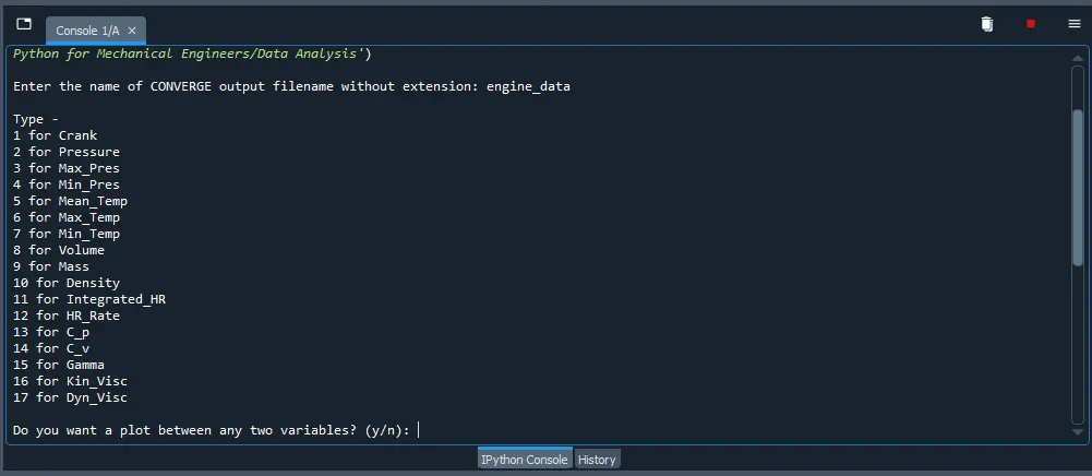
This part of the code allows the user to interactively select and plot any two variables from the parsed data.

# Displaying available variables for plotting
print('\nType -')
for i in a:
    print('{} for {}'.format(i, b[i - 1]))  # Displaying column indices and names

print('')
x = input("Do you want a plot between any two variables? (y/n): ")

# Interactive plotting loop
while x.lower() == 'y':
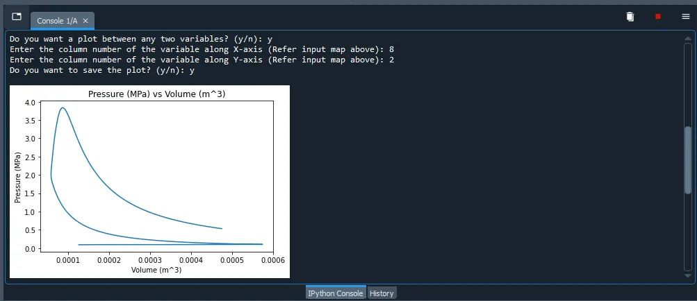
    cn1 = int(input("Enter the column number of the variable along X-axis (Refer input map above): "))
    cn2 = int(input("Enter the column number of the variable along Y-axis (Refer input map above): "))
    plt.figure()
    plt.plot(data[:, cn1 - 1], data[:, cn2 - 1])  # Plotting selected data
    plt.xlabel('{} {}'.format(b[cn1 - 1], c[cn1 - 1]))  # Labeling X-axis
    plt.ylabel('{} {}'.format(b[cn2 - 1], c[cn2 - 1]))  # Labeling Y-axis
    plt.title('{} {} vs {} {}'.format(b[cn2 - 1], c[cn2 - 1], b[cn1 - 1], c[cn1 - 1]))  # Setting plot title
    z = input("Do you want to save the plot? (y/n): ")
    if z.lower() == 'y':
        plt.savefig("{}-{}.png".format(b[cn2 - 1], b[cn1 - 1]))  # Saving plot
        plt.show()  # Displaying plot
        print('')
        x = input("\nDo you want to plot any other two variables? (y/n): ")  # Prompting for more plots
    else:
        plt.show()  # Displaying plot
        print('')
        break  # Exit the loop if the plot is not saved

• The available variables for plotting are displayed to the user with their corresponding indices.
• The user is prompted to choose whether to plot any two variables.
• Inside the interactive plotting loop:
  • The user is asked to input the column numbers of the variables to plot against each other.
  • A plot is generated using matplotlib.pyplot.plot() with the selected variables.
  • Labels for the x and y axes are set using the corresponding column names and units from the header.
  • The user is prompted to save the plot.
  • If the user chooses to save the plot, it is saved as a PNG file with a filename based on the selected variables.
  • The plot is displayed, and the user is prompted whether to plot any other two variables. If not, the loop breaks.

Engine Performance Analysis

This section calculates various engine performance metrics using the pressure and volume data from the CONVERGE output.

# Engine performance analysis
print('\nPERFORMANCE OF THE ENGINE')

# Finding columns for pressure and volume
b1 = [i.lower() for i in b]  # Converting column names to lowercase for case-insensitive search
pressure_column = b1.index('pressure')  # Finding pressure column index
volume_column = b1.index('volume')  # Finding volume column index

# Extracting pressure and volume data
pressure = data[:, pressure_column]  # Extracting pressure data
volume = data[:, volume_column]  # Extracting volume data

# Calculating work done per cycle (Area under P-V curve)
A = trapz(pressure, volume) * 1e6  # Calculating area under the curve

# Taking input from user for RPM and fuel consumption
rpm = float(input('\nEnter the rpm of the engine at which data was collected: '))
fuel_consumed_per_cycle = float(input('Enter the value of the fuel consumed per cycle (in micrograms): '))

# Calculating power output and specific fuel consumption
speed = (rpm / 60) / 2  # Converting rpm to cycles per second
P = A * speed  # Calculating power output
f = (fuel_consumed_per_cycle * rpm * 3600) / 1e9  # Converting micrograms to kilograms and adjusting for time
sfc = (f * 1000) / P  # Converting fuel consumption to kg/kW.hr

# Displaying results
print('\nArea under the P-V curve (Work done per cycle): {} J'.format(A))
print('\nPower output at {} rpm: {} kW'.format(rpm, P/1000))
print('\nSpecific fuel consumption: {} Kg/KW.hr'.format(sfc))

• This section begins by printing a header indicating engine performance analysis.
• It identifies the columns corresponding to pressure and volume data using a case-insensitive search.
• The pressure and volume data are extracted from the numpy array data.
• The work done per cycle (area under the P-V curve) is calculated using the trapezoidal rule (trapz function from scipy.integrate).
• The user is prompted to input the engine RPM and fuel consumption per cycle.
• Using the provided inputs and the calculated work done per cycle, the power output and specific fuel consumption are computed.
• Finally, the calculated metrics (work done, power output, and specific fuel consumption) are displayed to the user.

Plotting the P-V Curve

#Plotting area under PV
plt.plot(volume, pressure, color='blue', label='PV curve')
plt.fill_between(volume, pressure, color='lightblue', label='Area under curve')
plt.xlabel("Volume")
plt.ylabel("Pressure")
plt.legend()
plt.title("P-V Diagram and Area under Curve")
plt.savefig("area_under_PV_curve.png")
plt.show()

• This section plots the P-V curve using the extracted pressure and volume data.
• It uses matplotlib.pyplot.plot() to plot the P-V curve with blue color.
• The area under the curve is highlighted using matplotlib.pyplot.fill_between() with light blue color.
• Labels, legend, and title are added to the plot.
• The plot is saved as "area_under_PV_curve.png" and displayed to the user using plt.show().

Output:

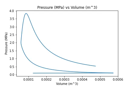
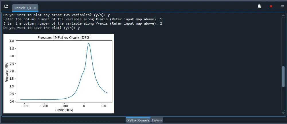
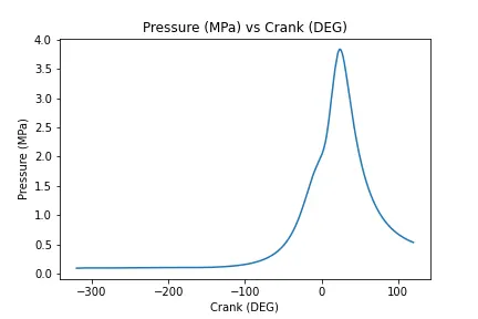
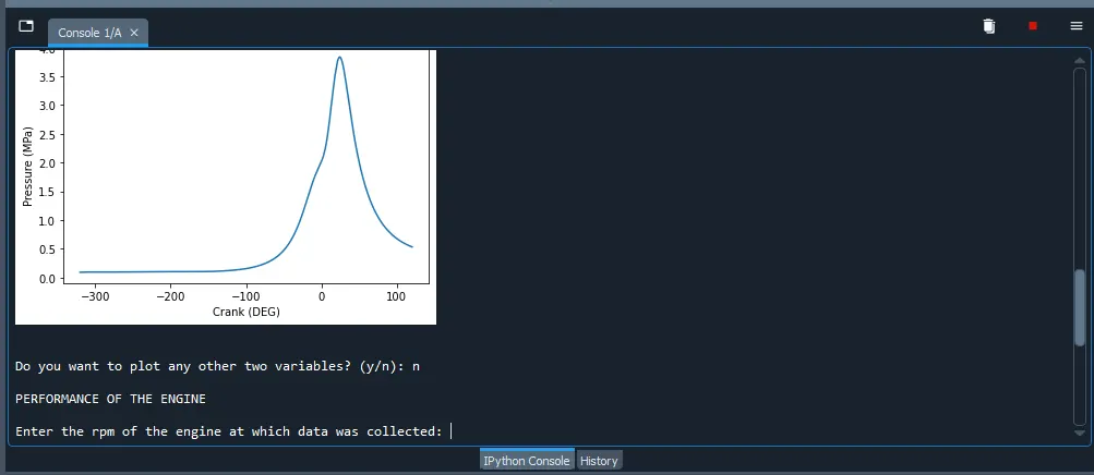
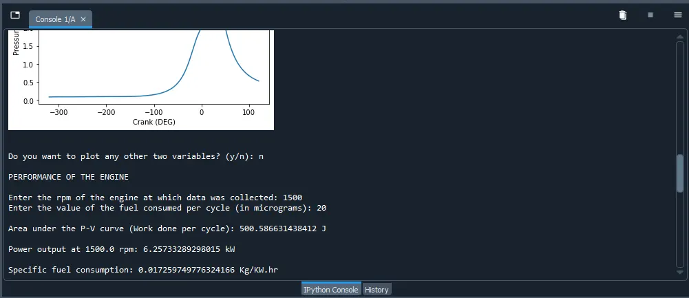
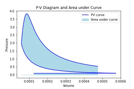
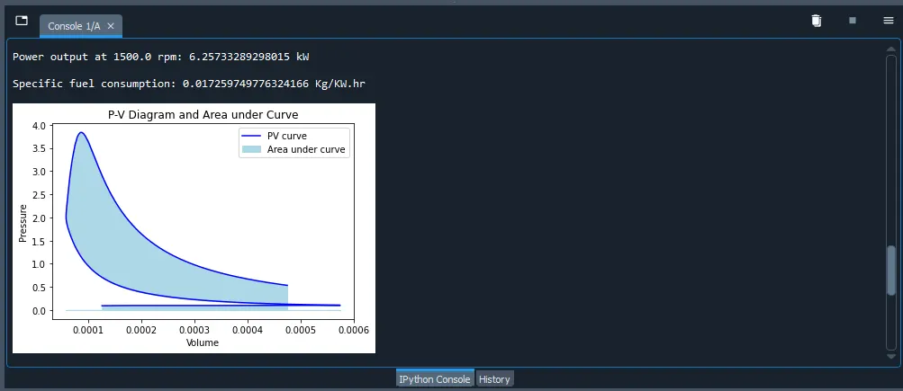
Area under the P-V curve (Work done per cycle): 500.586631438412 J

Power output at 1500.0 rpm: 6.25733289298015 kW

Specific fuel consumption: 0.017259749776324166 Kg/KW.hr

Error:

While entering the wrong filename,

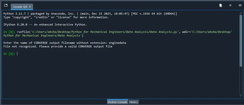
While entering a filename with no data,

Conclusion:

In conclusion, this analysis provides valuable insights into the performance of the engine based on CONVERGE output data. By analyzing the P-V curve, we determined the work done per cycle, enabling us to calculate the engine's power output and specific fuel consumption. The interactive plotting feature facilitates visual exploration of various variables, enhancing understanding. These findings offer crucial information for optimizing engine performance and fuel efficiency. Overall, this report serves as a comprehensive assessment tool for evaluating and improving engine operation.

Note: I have attached a sample empty file named 'data.out' in the zip folder for a compatability check (with no data).