Week 3 - Taylor table method and Matlab code

AIM :

Taylors table method

THEORY:

The taylors series for a function is written as :

`f(x+deltax) = f(x) + delf/delx*deltax + del^2f/delx^2*(deltax^2/2) + ....`----(1)

the above equation is only valid if :

• if the number of terms is infinite and the series converges
• `deltax` tends to zero.

If u(i,j) is the x component velocity at point (i,j) ; u(i+1,j) is x component velocity at point (i+1,j) then from equation 1:

`u(i+1,j) = u(i,j) + delu/delx(i,j)*deltax+del^2u/delx^2(i,j)*(deltax^2/2)+....`----(2)

solving for `delu/delx(i,j)` we get ;

`delu/delx(i,j) = (u(i+1,j)-u(i,j))/deltax - del^2u/delx^2(i,j)*(deltax/2)+...`-------(3)

The term in the RHS of equation 3 containing u(i+j) -u(i,j) is the finite difference . The other terms that are neglected is the truncation error.

Since in majority of the CFD , first order approximation is not sufficient. We turn our heads to central difference schemes .

`del^2u/delx^2= (u(i+j,j)-2*u(i,j)+u(i-j,j))/(deltax^2) + errors`

Taylors table is a method that comes up with schemes that meet the targetted accuracy .

The formula for number of nodes is as follows :

• for the central differences scheme , number of nodes = p+q-1 , where p is the order of derivative and q is the order of approximation .
• for the skewed schemes , be it right sided ar left sided , the number of nodes is p+q , where p is the order of derivative and q is the order of approximation .

Since the order is second and the order of approximation is 4 , the number of nodes in central difference scheme is 5 and number of nodes is skewed right sided and skewed left sided schemes is 6 .

CENTRAL DIFFERENCING SCHEME :

We take up a hypothetical equation like :

`del^2u/delx^2 = a*f(i-2)+b*f(i-1) + c*f(i) +d*f(i+1) +e*f(i+2)`-----------(5)

Here the a,b,c,d,e are coefficients , The values of these coefficients are needed to be found out . The mode of operandi will be like this. :

• Firstly we expand the every term of the above equation according to Taylors series.
• Then we write the values obtained in a table format . The columns are the stencils.
• Then we equate the equtions with unknowns to find out the values .

From equation 5 :

`a*f(i-2) = a*f(i) + a*delu/delx*(-2*deltax/1) + a*del^2u/delx^2*((-2*deltax)^2/4)) +a*del^3u/delx^3*((-2*deltax)^3/6) + a*del^4u/delx^4*((-2*deltax)^4/24)`---------(6)

`b*f(i-1) = b*f(i) + b*delu/delx*(-deltax/1) + b*del^2u/delx^2*((-deltax)^2/2) +b*del^3u/delx^3*((-deltax)^3/6) + b*del^4u/delx^4*((-deltax)^4/24)/`---------------------(7)

`c*f(i) = c*f(i)`--------(8)

`d*f(i+1) = d*f(i) + d*delu/delx*deltax + d*del^2/delx^2*((deltax)^2/2) + d*del^3u/delx^3*((deltax)^3/6) + d*del^4u/delx^4*((deltax)^4/24)`-------------------(9)

`e*f(i+2) = e*f(i) + e*delu/delx*(2*deltax) + e*del^2u/delx^2*((2*deltax)^2/2) + e*del^3u/delx^3*((2*deltax)^3/6) + e*del^4u/delx^4*((2*deltax)^4/24)`------(10)

re arranging , we get :

`del^u/delx^2 = f(i)(a+b+c+d+e) + delu/delx*deltax*(-2*a+(-b) +d +2*e) +del^2u/delx^2*(deltax^2)*(2*a + b/2 +d/2 +2*e) + del^u/delx^3*(deltax^3)*(-(8/6)*a+(-b/6)+d/6 +8*e/6) + del^4u/delx^4*deltax^4*(16*a/24 + b/24 + d/24 +16*e/24)`---------(11)

If the equation 11 is written in tabular form , we get the Taylors table as :

	f(i)	`delu/delx*deltax`	`del^u/delx^2*deltax^2`	`del^3u/delx^3*deltax^3`	`del^4u/delx^4*deltax^4`
`a*f(i-2)`	a	-2*a	2*a	-(8*a/6)	16*a/24
`b*f(i-1)`	b	-b	b/2	-(b/6)	b/24
`c*f(i)`	c	0	0	0	0
`d*f(i+1)`	d	d	d/2	d/6	d/24
`e*f(i+2)`	e	2*e	2*e	(8/6)*e	16/24*e

Approximating and adding up the coefficients with the logic that the term f(i), `delu/delx`, `del^3u/delx^3`,`del^4u/delx^4` will be approximated to zero and the term `del^2u/delx^2`will be approximated to 1 , we gt the following set of equations :

a + b+ c+ d + e = 0

-2*a -b +d + 2*e = 0

2*a +b/2 + d/2 +2*e = 1

-(8/6)*a - b/6 +d/6 +(8*e/6) = 0

16/24*a + b/24 + d/24 + 16*e/24 = 0

Writing in a matrix form :

`[[1,1,1,1,1],[-2,-1,0,1,2],[2,1/2,0,1/2,2].[-8/6,-1/6,0,1/6,8/6].[16/24,1/24,0,1/2416/24]` *`((a),(b),(c),(d))` = `((0),(0),(1),(0),(0))`

Solving the above equation we get , a= (-1/12) ; b= (4/3) ; c = (-5/2); d = (4/3); e = (-1/12)

So by putting the above values of the coefficients in the main equation :

`del^2u/delx^2 = (-1/12)*f(i-2) +(4/3)*f(i-1) + (-5/2)*f(i) + (4/3)*f(i+1) + (-1/12)*f(i+2)`-----(**)

Now for skewed right sided and skewed left sided schemes the same above way is followed to create the Taylors table. here we directly input the table by not repeting the procedure:

SKEWED RIGHT SIDED DIFFERENCE :

The hypothetical equation is ;

`del^2u/delx^2 = a*f(i) + b*f(i+1) +c*f(i+2) +d*f(i+3) +e*f(i+4) +g*f(i+5)`

Expanding each of the above terms in the order of taylors series ; We obtain the Taylors table as :

	f(i)	`delu/delx*deltax`	`del^u/delx^2*(deltax)^2`	`del^3u/delx^3*(deltax)^3`	`del^4u/delx^4*(deltax)^4`	`del^5u/delx^5*(deltax)^5`
a*f(i)	a	0	0	0	0	0
b*f(i+1)	b	b	b/2	b/6	b/24	b/120
c*f(i+2)	c	2*c	2*c	8/6*c	16/24*c	32/120*c
d*f(i+3)	d	3*d	9/2*d	27/6*d	81/24*d	243/120*d
e*f(i+4)	e	4*e	8*e	64/6*e	256/24*e	1024/120*e
g*f(i+5)	g	5*g	25/2*g	125/6*g	625/24*g	3125/120*g

Solving the above equations by applying the same logic that the term containg second order derivative is approximated to 1 and all others to zero we get the coefficients as :

a = (15/4); b =(-77/6); c=(107/6); d = -13 ; e = (61/12); g = (-5/6)

Putting the values in the parent equation we get :

`del^u/delx^2 = (15/4)*f(i) + (-77/6)*f(i+1) + (107/6)*f(i+2) +(-13)*f(i+3) +(61/12)*f(i+4) + (-5/6)*f(i+5)`

SKEWED LEFT SIDED DIFFERENCE:

In this scheme we will consider the discretization points at the left side . The hypothetical equation for this scheme is written as :

`del^2u/delx^2 = a*f(i) + b*f(i-1) + c*f(i-2) +d*f(i-3) + e*f(i-4) +g*f(i-5)`

By expanding each and every terms of the RHS according to the taylors series we get :

`a*f(i) = a*f(i)`

`b*f(i-1) = b*f(i) + b*delu/delx*(-deltax) + b*del^2u/delx^2*((-deltax)^2/2)+b*del^3u/delx^3*((-deltax)^3/6) +b*del^4u/delx^4*((-deltax)^4/24) + b*del^5u/delx^5*((-deltax)^5/120)``

`c*f(i-2) = c*f(i) + delu/delx*c*((-2*deltax)) + c*del^2u/delx^2*((-2*deltax)^2/2) + c*del^3u/delx^3*((-2*deltax)^3/6) + c*del^4u/delx^4*((-2*deltax)^4/24) + c*del^5u/delx^5*((-2*deltax)^5/120)`

`d*f(i-3) = d*f(i) + d*delu/delx*((-3*deltax)) + d*del^2u/delx^2*((-3*deltax)^2/2)+d*del^3u/delx^3*((-3*deltax)^3/6) + d*del^4u/delx^4*((-3*deltax)^4/24) + d*del^5u/delx^5*((-3*deltax)^5/120)`

`e*f(i-4) = e*f(i) +e*delu/delx*((-4*deltax) + e*del^2u/delx^2*((-4*deltax)^2/2) + e*del^3u/delx^3*((-4*deltax)^3/6) +e*del^4u/delx^4*((-4*deltax)^4/24) + e*del^5u/delx^5)*((-4*deltax)^5/120`

`g*f(i-5) = g*f(i) + g*delu/delx*(-5*deltax) + g*del^u/delx^2*((-5*deltax)^2/2) + g*del^3u/delx^3*((-5*deltax)^3/6) + g*del^4u/delx^4*((-5*deltax)^4/24) + g*del^5u/delx^5*((-5*deltax)^5/120)`

By rearranging the above equations ,

	f(i)	`delu/delx*(deltax)`	`del^2u/delx^2*((deltax)^2)`	`del^3u/delx^3*((deltax)^3)`	`del^4u/delx^4*((deltax)^4)`	`del^5u/delx^5*((deltax)^5)`
a*f(i)	a	0	0	0	0	0
b*f(i-1)	b	-b	b/2	-b/6	b/24	-b/120
c*f(i-2)	c	-2c	2c	-8/6*c	16/24*c	-32/120*c
d*f(i-3)	d	-3d	9/2*d	-27/6*d	81/24*d	-243/120*d
e*f(i-4)	e	-4e	8e	-64/6*e	256/24*e	-1024/120*e
g*f(i-5)	g	-5g	25/2*g	-125/6*g	625/24*g	-3125/120*g

in matrix form the equation stands as :

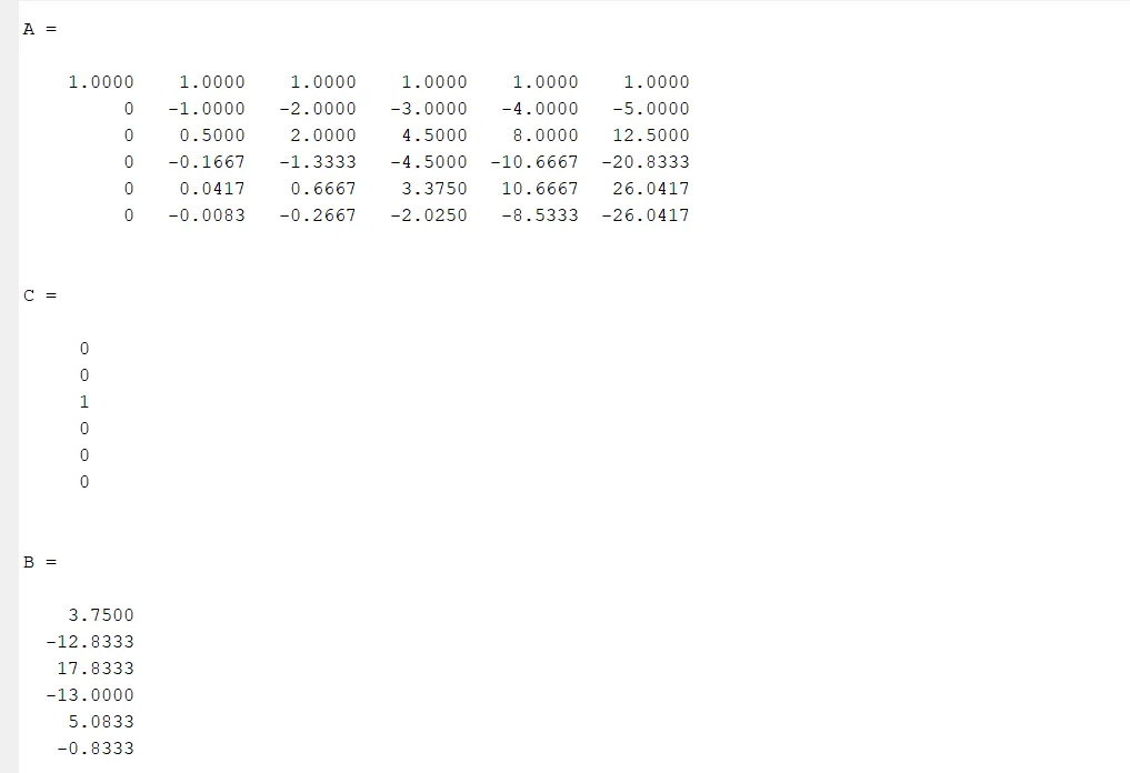
`[[1,1,1,1,1,1],[0,-1,-2,-3,-4,-5],[0,1/2,2,9/2,8,25/2],[0,-1/6,-8/6,-27/6,-64/6,-125/6],[0,1/24,16/24,81/24,256/24,625/24],[0,-1/120,-32/120,-243/120,-1024/120,-3125/120]`*`((a),(b),(c),(d),(e),(g))` = `((0),(0),(1),(0),(0),(0))`

Solving it by matrix inversion method in matlab , we get the coefficients as :

a = 3.75;b= -12.8333;c=17.8333;d=-13.000; e= 5.083;g = -0.8333

Putting the values of the coefficents :

`del^2u/delx^2 = 3.75*f(i) + (-12.8333)*f(i-1) +17.8333*f(i-2)+(-13)*f(i-3)+5*f(i-4)+(-0.8333)*f(i-5)`

Matrix repesentation of the above case is provided. same is followed for the other two schems :

CODING EXPLANATION :

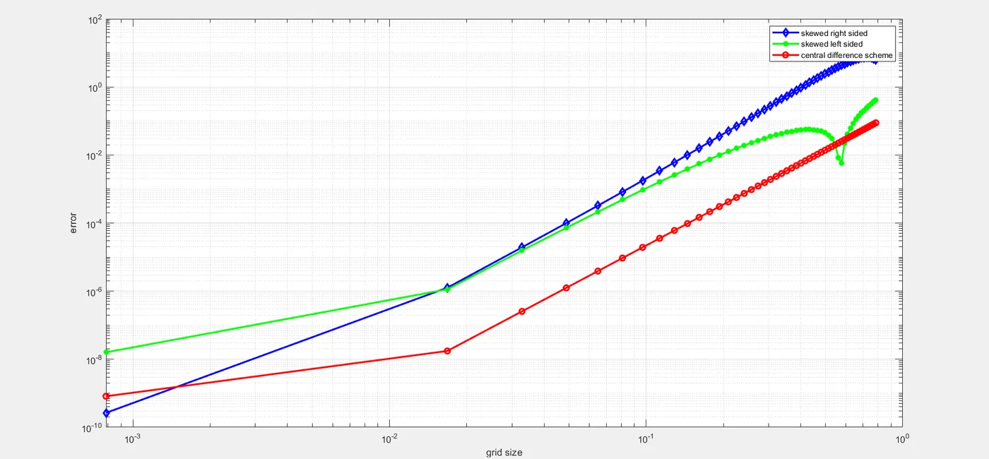
our aim is to compare the errors calculated through the three different schemes .

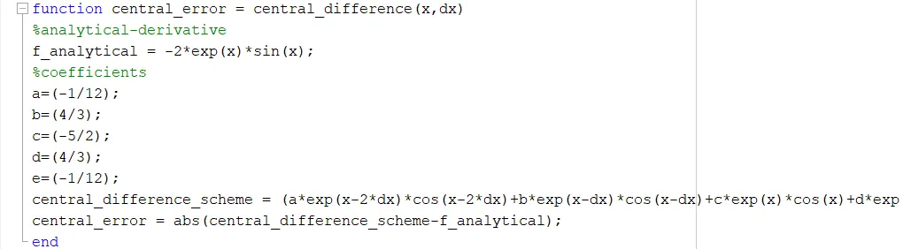
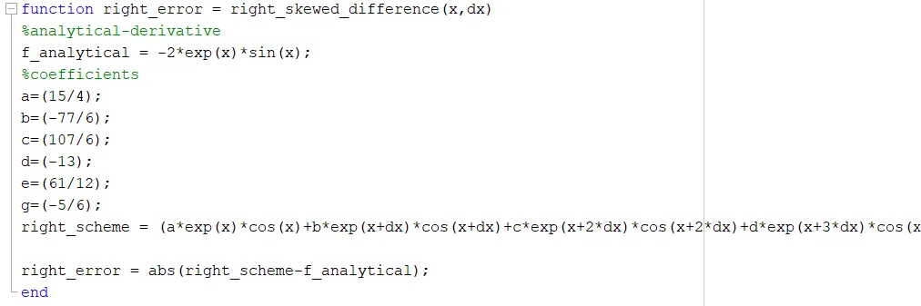
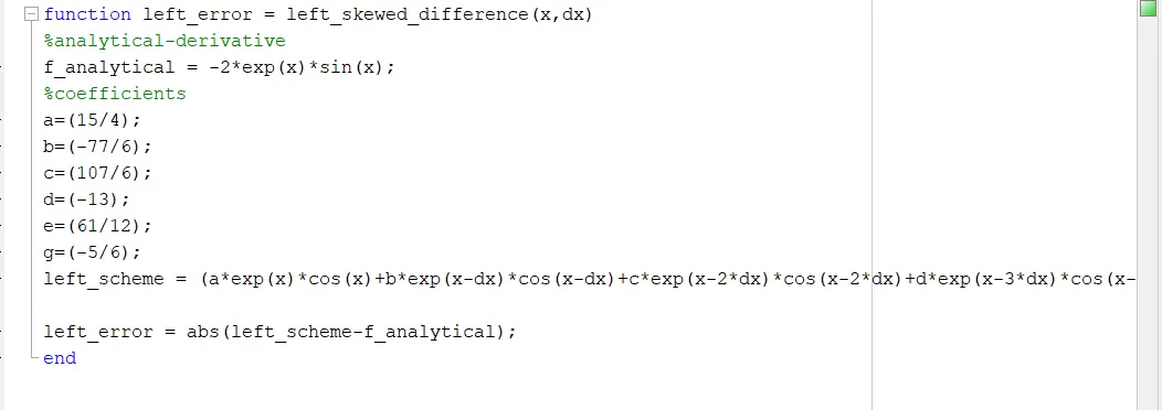
• The function code is written for the three different schemes , the use of a function icode is that we can call that value again and again in a main body. Care is taken for the syntaxes of a function. The coefficient values are provided that are obtained through the matrix inversion method by solving the linear equations above. The analytical derivative value is calculated. since it is of second order , thje second derivative is calculated. The error is calculated by using the abs command and subtracting the analytical derivative function from the three different schemes .

• In the main body , there is basically three parts ; First one is assigning the value of x, the range of dx . The linspace command is used to provide input for the dx as we intend to create an array that will store the dx values between two limits . dx is bvasiccaly the grit size or the mesh size. Second one is creating a for loop . the main idea behind the for loop is that we want to calculate the errors for the three different schemes throughout the range of dx values . i is the loop counter variable. it keeps on updating. Third one is creating a plot. A loglog plot is created , proper lables are given using xlabel and ylabel.

MATLAB CODE:

clear all 
close all 
clc

%analytical_function = exp(x)*cos(x)
%analytical_derivative = -2*exp(x)*sin(x)
x = pi/3;
dx=linspace(pi/4000,pi/4,50);%range of dx that is mesh size 
%a for loop to calculatr error through the range of dx 
for i = 1:length(dx)
    
    central_difference_scheme_error(i) = central_difference(x,dx(i));
    skewed_right_sided_scheme_error(i) = right_skewed_difference(x,dx(i));
    skewed_left_sided_scheme_error(i) = left_skewed_difference(x,dx(i));
    
    
end

%plotting the errors
figure(1)

loglog(dx,skewed_right_sided_scheme_error,'linewidth',2,'color','b','marker','diamond')
hold on
loglog(dx,skewed_left_sided_scheme_error,'linewidth',2,'color','g','marker','*')
hold on
loglog(dx,central_difference_scheme_error,'linewidth',2,'color','r','marker','o')
grid on
xlabel('grid size')
ylabel('error')
legend('skewed right sided','skewed left sided','central difference scheme')

FUNCTIONS CODE:

function left_error = left_skewed_difference(x,dx)
%analytical-derivative
f_analytical = -2*exp(x)*sin(x);
%coefficients 
a=(15/4);
b=(-77/6);
c=(107/6);
d=(-13);
e=(61/12);
g=(-5/6);
left_scheme = (a*exp(x)*cos(x)+b*exp(x-dx)*cos(x-dx)+c*exp(x-2*dx)*cos(x-2*dx)+d*exp(x-3*dx)*cos(x-3*dx)+e*exp(x-4*dx)*cos(x-4*dx)+g*exp(x-5*dx)*cos(x-5*dx))/(dx^2);

left_error = abs(left_scheme-f_analytical);
end

function right_error = right_skewed_difference(x,dx)
%analytical-derivative
f_analytical = -2*exp(x)*sin(x);
%coefficients 
a=(15/4);
b=(-77/6);
c=(107/6);
d=(-13);
e=(61/12);
g=(-5/6);
right_scheme = (a*exp(x)*cos(x)+b*exp(x+dx)*cos(x+dx)+c*exp(x+2*dx)*cos(x+2*dx)+d*exp(x+3*dx)*cos(x+3*dx)+e*exp(x+4*dx)*cos(x+4*dx)+g*exp(x+5*dx)*cos(x+5*dx))/(dx^2);

right_error = abs(right_scheme-f_analytical);
end

function central_error = central_difference(x,dx)
%analytical-derivative
f_analytical = -2*exp(x)*sin(x);
%coefficients 
a=(-1/12);
b=(4/3);
c=(-5/2);
d=(4/3);
e=(-1/12);
central_difference_scheme = (a*exp(x-2*dx)*cos(x-2*dx)+b*exp(x-dx)*cos(x-dx)+c*exp(x)*cos(x)+d*exp(x+dx)*cos(x+dx)+e*exp(x+2*dx)*cos(x+2*dx))/(dx^2);
central_error = abs(central_difference_scheme-f_analytical);
end

OUTPUT:

CONCLUSION:

For a same value of dx , the central difference scheme gives minimum error than the other two schemes .

• For right sided skewed scheme , we take points nodes right of the point. For left sidede skewed scheme we take nodes left of the point.
• In CFD , first order accuracy is not sufficient. We require second orer accuracy.
• The main demerit of a higher order accuracy is that more grid points are required , so more computng time.
• Higher order accuracy gives more qualitative solution.
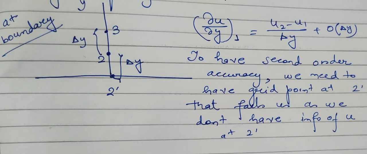
• the skewed schemes finds its importance in the discretization in boundaries.If we tend to apply central difference scheme at the boundary , we will need to have information about the parameter at a point below the boundary that we dont have. Refection method was used earlier that is of little help. skewed schemes finds its importance there.