Week 6: Conjugate Heat Transfer Simulation

Aim: - To perform a transient state Conjugate Heat Transfer (CHT) simulation for Pipe flow using Converge.

Objective: -

• To setup a CHT simulation for grid sizes [2 mm, 3 mm, 4 mm] with using Super-Cycling feature for flow of Reynold’s Number equal to 7000.
• To setup a CHT simulation for 3 mm grid size with using Super-Cycling feature with 3 different time lengths [0.01, 0.02, 0.03] sec for Super-cycle stage.
• Plot and compare the results for grid, Temperature and Velocity Contours, Y+ using Converge and ParaView.

Theory: -

Conjugate Heat Transfer (CHT) –

Conjugate heat transfer (CHT) analysis can accurately predict heat transfer by simultaneous solving all the relevant solid and flow field heat transfer processes.

It allows for the simulation of heat transfer between solid and fluid domains by exchanging thermal energy at the interfaces between them, which is more stable and provides faster convergence as the energy equation is strongly coupled between the solid and fluid regions.

It is preferred over Finite Element Thermal analyses for wall heat transfer coefficients and their local variations on surfaces are directly calculated within the model rather than based on simplified empirical calculations. The CHT approach therefore has benefits for those applications where heat transfer is either non-uniform or difficult to calculate empirically.

Used in Thermal analysis of –

• Systems – HVAC, Automotive etc
• Electronic Devices for Heat Dissipation analysis
• Mechanical Components – Turbochargers, Combustor, Burners etc.
• Power Plants.

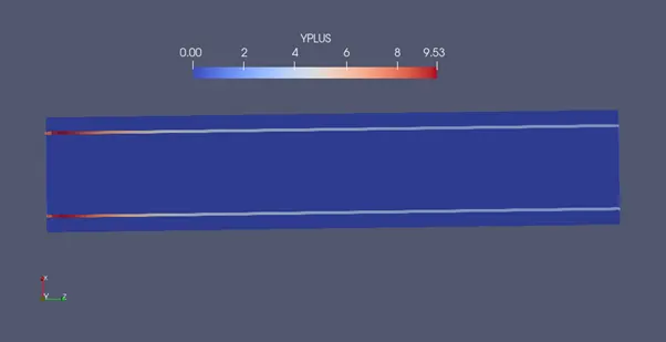
Y+

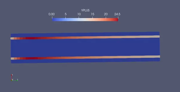
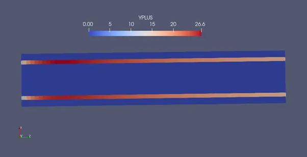
It is a non-dimensional distance. It is often used to describe how coarse or fine a mesh is for a particular flow pattern. It is important in turbulence modelling to determine the proper size of the cells near domain walls.

It is undesirable to have Y+ between 10 and 30 as modelling the transition between laminar and turbulent. Y+ less than 10 is laminar region while above 30 it is turbulent region.

Introduction: -

A pipe-flow simulation is setup with heat input of 10,000 W/m² to outer wall of pipe and for flow of 7000 Reynold’s Number. The inlet velocity is calculated by following formulae –

`Re = (ρ*V*D)/(μ)`

where `rho` is density at 300 K is 1.161 Kg/m³, D is characteristics length (Diameter) = 0.03 m

µ is dynamic Viscosity at 300 K is 1.81e-5 Pa-sec.

On substituting the values, we get, inlet velocity = 3.64 m/sec

A: The simulation is run for three mesh sizes starting from base to refined mesh, sizes are –

• case 1: dx = 0.004 m, dy = 0.004 m dz = 0.004 m
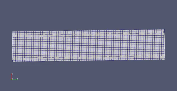
• case 2: dx = 0.003 m, dy = 0.003 m dz = 0.003 m
• case 3: dx = 0.002 m, dy = 0.002 m dz = 0.002 m

for above all cases the super cycling interval is set at 0.05 sec

B: The simulation is run for mesh size of 0.003 m for following super cycling intervals [0.01, 0.02, 0.03] sec.

Geometry Model –

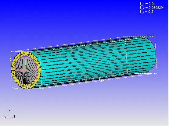
The inner radius is 0.015 m and the outer radius is 0.02 m. The length of pipe is 0.2 m.

Case Setup –

1. Time Based application type.
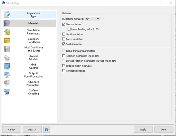
2. Gas and Solid simulation with Air as predefined mixture and Aluminum as solid pipe.

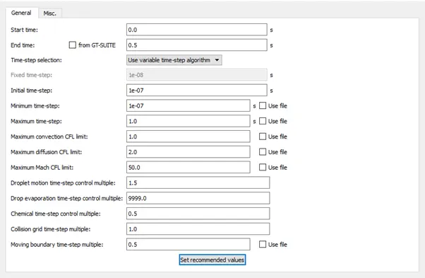
3. Density Based Transient State Solver is used with Compressible Gas Flow solver and PISO Navier-Stokes’s solver scheme.
4. The solution run for 0.5 sec with minimum time step of 1e-7 sec and maximum up to 1 sec.

5. Boundary Condition:
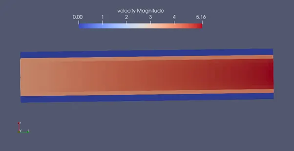
   3. Inlet - Type = Inflow, Region = Fluid region, Pressure = Zero normal gradient, Velocity = 3.64 m/sec in z direction, Temperature = 300 K, Species = O2:0.23, N2: 0.77
   4. Outlet - Type = outflow, Region = Fluid region, Pressure and Velocity = 101325 Pa, Temperature = 300 K Species = O2:0.23, N2: 0.77
   5. Solid-thickness – Type = wall, Region = Solid region, slip Condition
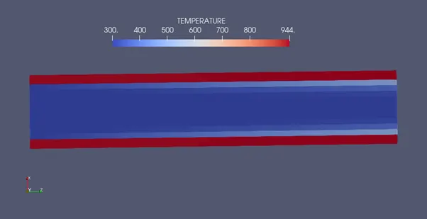
   6. Solid-outer-wall – Type = wall, Region = Solid region, slip Condition, Temperature BC = heat flux [-10,000 W/m²]
   7. Interface – Type = interface, forward = Fluid region, Reverse = Solid region
6. Fluid Region is initialized with Temperature 300, Pressure 101325 Pa and mass fraction of O2: 0.23 and N2: 0.77.

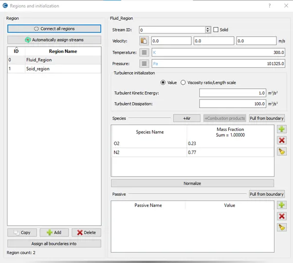
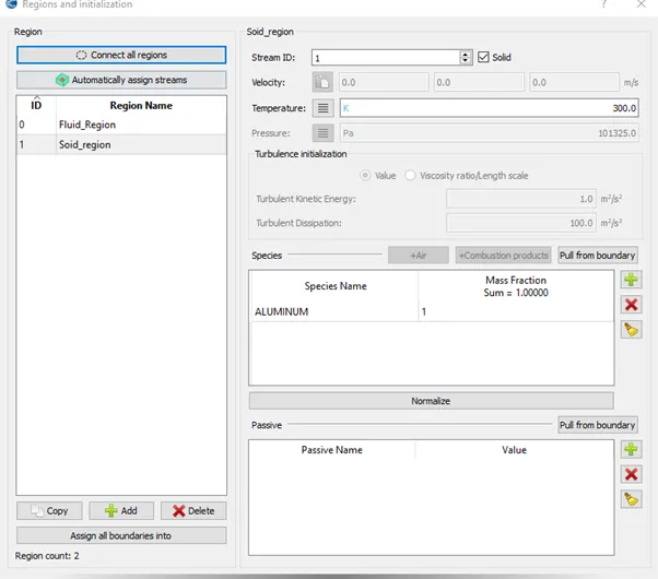
7. Solid Region is initialized with Stream ID = 1, Species = Aluminum.

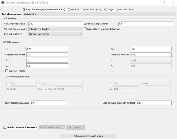
8. Realizable K-epsilon is used for turbulence modelling with recommended values.

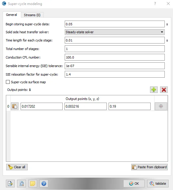
9. Super-Cycling model is used for solid side heat transfer with 0.05 sec as super-cycling interval. A point is set at just before the Outlet for output point.
10. Base grids of 0.004 m or other for respective cases are generated for all axis.
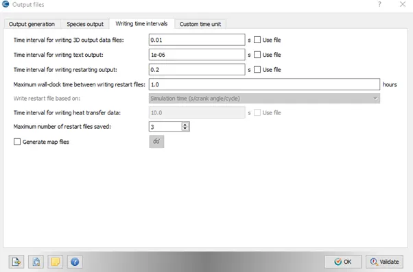
11. Y+ value is checked in post variable output. 3D output data is written after every 0.01 sec.

12. The input files are exported to a folder to further solving.

Solving using Cygwin:

An executable “mpiexec.exe” is placed with the exported folder. The Cygwin directory is navigated to the above saved folder and following code is entered to solve the problem.

mpiexec.exe -n 2 "C:\Program Files\Convergent_Science\CONVERGE\3.0.16\bin\intelmpi\converge.exe" restricted </dev/null> logfile &

where address in quotes gives the path of folder containing input file exported earlier.

Post-Processing:

Post-Processing is done with the help of Converge CFD post processing tab –

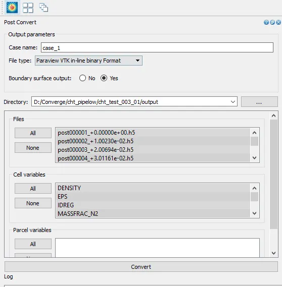
with these the output 3D data is converted in ‘. vtm’ file and contours and animations are prepared though ParaView.

Results: -

PART A:

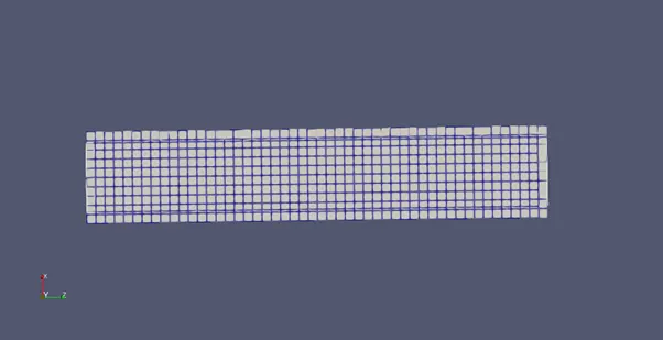
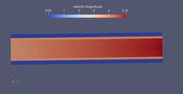
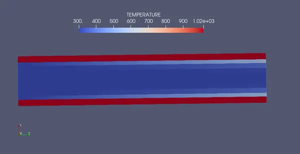
case 1 – dx = 0.004 m, dy = 0.004 m dz = 0.004 m

Mesh

Velocity Contour

Temperature Contour

Y+ contour

case 2 – dx = 0.003 m, dy = 0.003 m dz = 0.003 m

Mesh

Velocity Contour

Temperature Contour

Y+ contour

case 3 – dx = 0.002 m, dy = 0.002 m dz = 0.002 m

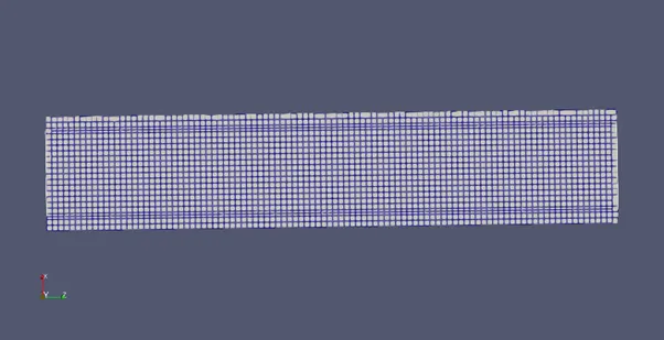
Mesh

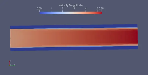
Velocity Contour

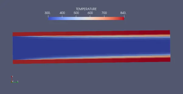
Temperature Contour

Y+ contour

Comparison Between above cases

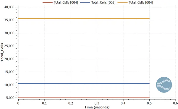
Total cell count

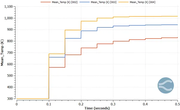
mean Temperature

PART B:

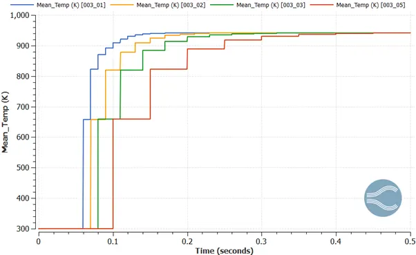
Mean Temperature

Conclusion: -

1. As the flow is in turbulent region the Y+ should be above 30 and hence the 3 mm grid size with 0.02 super-cycling interval give better result as Y+ is equal to 51.
2. The plots with grid size 3 and 4 are fairly closer as they are in transition stage while 2 mm grid size belongs to laminar.
3. As the Super-cycling interval decreases the accuracy increases and calculation time decreases as solution converges fast.