Week 6: Conjugate Heat Transfer Simulation

Objective:

• Setting up a flow simulation through a pipe
• Inlet Reynolds number should be 7,000
• Turbulence modelling - K-Epsilon
• To study the effect of supercycling

Introduction:

Conjugate heat transfer is when heat transfer occurs simultaneously within and between fluid and solid regions.

The predominant mode of heat transfer in fluids is convection. the predominant mode of heat transfer in solids is conduction.

Converge solves the fluid heat transfer using energy equation.

Converge solves the solid heat equation :

`c_p*rho*(delT)/(delt)=nabla*(k*nablaT)+S_h`

In the above equation, `c_p`is the specific heat capacity at constant pressure. `rho`is the density of the solid. `k` is the thermal conductivity of the solid. `S_h`is the energy source if any.

CFD modelling:

The CFD modelling of the CHT analysis includes the following steps:

• Proper defining the fluid and solid materials and their physical properties.
• Configuration of fluid and solid regions
• Assignment of regions to streams
• Using approximate Boundary conditions
• Selection of time control methods (Supercycle)
• Post processing the results.

1) Applicatiin type:

The application type is time based. The time is measured in seconds.

2) Material selection:

Predefined mixture is air. gas simulation and solid simulation both is selected.

Solid set up:

Temperature dependent solid properties is defined in the converge studio. case set up>Materials>Solid simulation

One or more solid species can be defined.

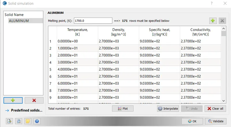
The gas simulation and the global transport parameters are kept as provided by default .

Under species, Gas - O2 and N2 are selected. And under the solid , Aluminium is selected.

This concludes the material set up.

3) Simulation parameters:

• Run parameters:

Solver : Transient

Simulation mode : Full Hydrodynamic

Gas flow solver : Compressible

temporal type : Time based simulation

• Simulation time parameters:

Start time : 0 secs

End time: 0.7 secs

Initial time step: 1e-9

Minimum time step: 1e-9

Maximum time step: 1

Maximum Convection CFL limit:1

Maximum diffusion CFL limit:2

• Solver parameters:

The Navier stokes solver scheme is PISO and the solver type is Density based.

Other parameters are default selections.

4) Boundary conditions:

• Inner wall :

Boundary type : Interface .

Interface boundary is the boundary that separates two types of materials or phases. Conjugate heat transfer requires atleast one interface boundary. An interface boundary demarcates two different material or phases.

Boundary condition for forward and reverse boundary of each interface must be defined.

The boundary facing the direction of the normal vector is the forward boundary.

The boundary facing the opposite direction of the normal vectors is the reverse boundary.

Wall motion type is stationary and the contact resistence is 0.Contact resistence 0 means at the interface the temperature is continuous.

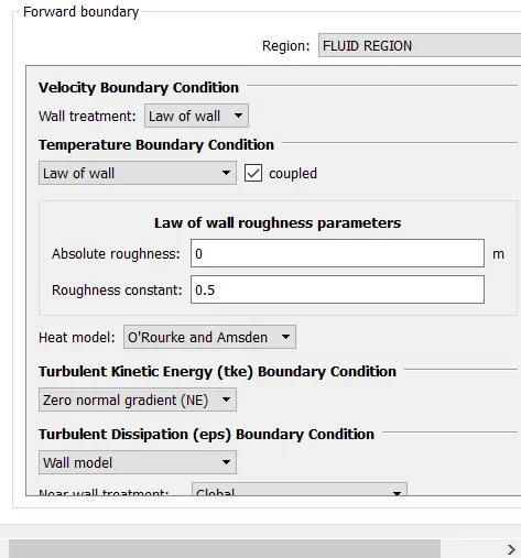
The forward side has the fluid region assigned to it.

Wall treatment follows law of the wall. Temperature boundary conditions also follow the law of the wall and is coupled.

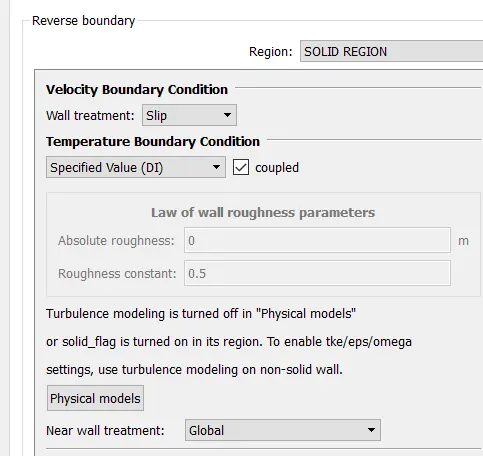
The reverse boundary has the solid region assigned to it. Wall treatment is slip And the temperature boundary condition is Specifiued value(DI) and coupled.

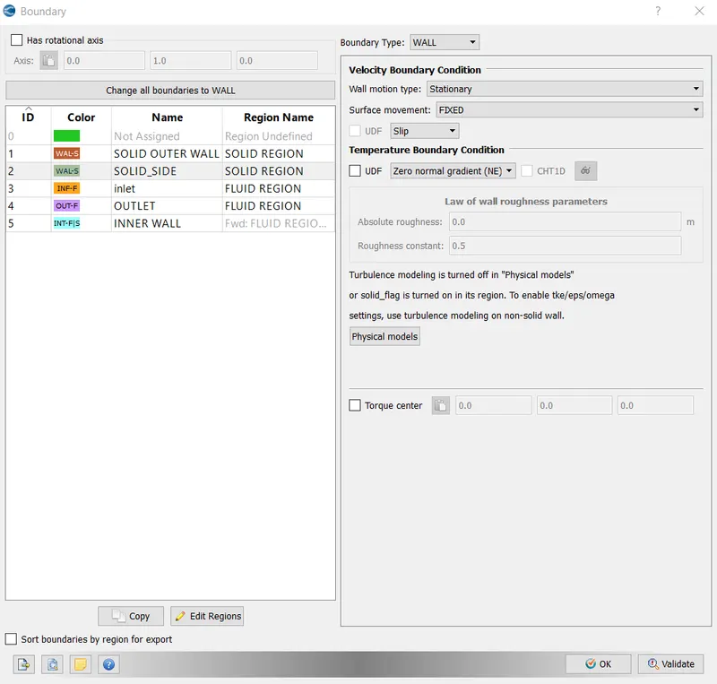
• Solid outer wall:

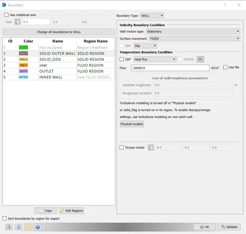
The boundary type is wall.

The wall motion type is stationary and the surface movement is fixed. Slip conditon is applied.

The temperature boundary conditions allwed are :

Dirichlet: Specifying the wall temperature directly

heat flux: Specifying the heat flux per surface area of the boundary. In case of a negative value of the heat flux, it signifies that the energy is entering the solid. In case of positive value, the energy exits the system.

Convection: Specifying the heat transfer coefficient and a far field temperature.

In this case ,the heat flux is pecified as (-20000)W/m^2 . the energy is entering the solid.

• Solid side :

The boundary type is wall.

This side is basically adiabatic in nature.

Under the velocity boundary conditions, The wall motion type is stationary and the surface movement is fixed. Slip condition prevails. the temperature boundary condition is Zero normal gradient(NE)

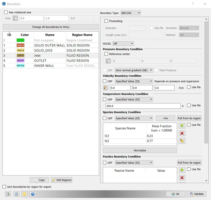
• Inlet:

The bumdary type is inflow.

Oressure boundary conditions: Zero Normal gradient (NE)

Velocity boundary conditions: specified value (DI)

The z velocity :

`re=(rho*V*D)/(mu)`

where, the `rho,V,D,mu` are the density of the fluid, Velocity of the flow, Characteristic dimension of the cylinder and the dynamic viscosity of the fluid.

here the valuse are:

`rho`= 1.225 kg/m^3

`mu`=1.81*10^-5 N-s/m^2

`V` this value is calculated from the above equation, keeping the value of reynolds number to 7000.

`V`= 3.59 that is nearly equal to 3.6 m/s

The temperature boundary condition is specified value DI. specified at 300 K

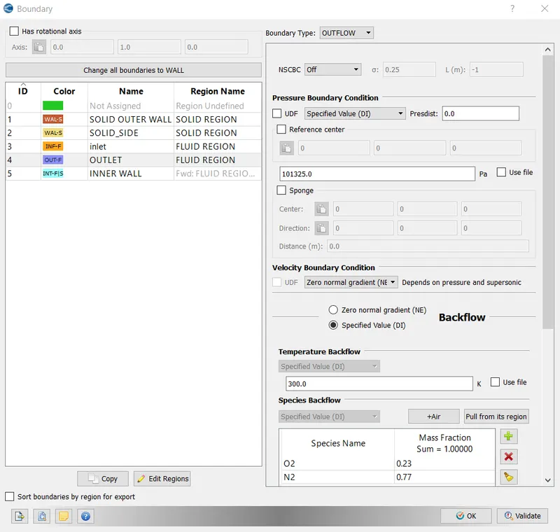
• Outlet :

Boundary type : outflow.

The pressure boundary condition is specified value at 101325 pas.

the velocity boundary condition is Zero normal gradient(NE).

5) Regions and initializations:

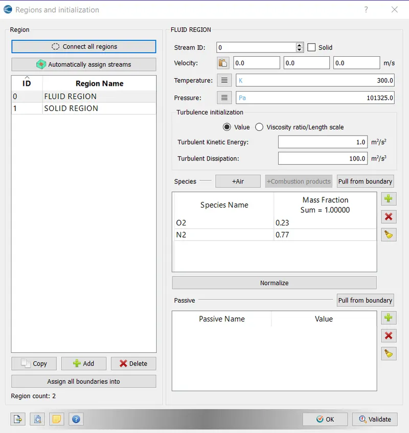
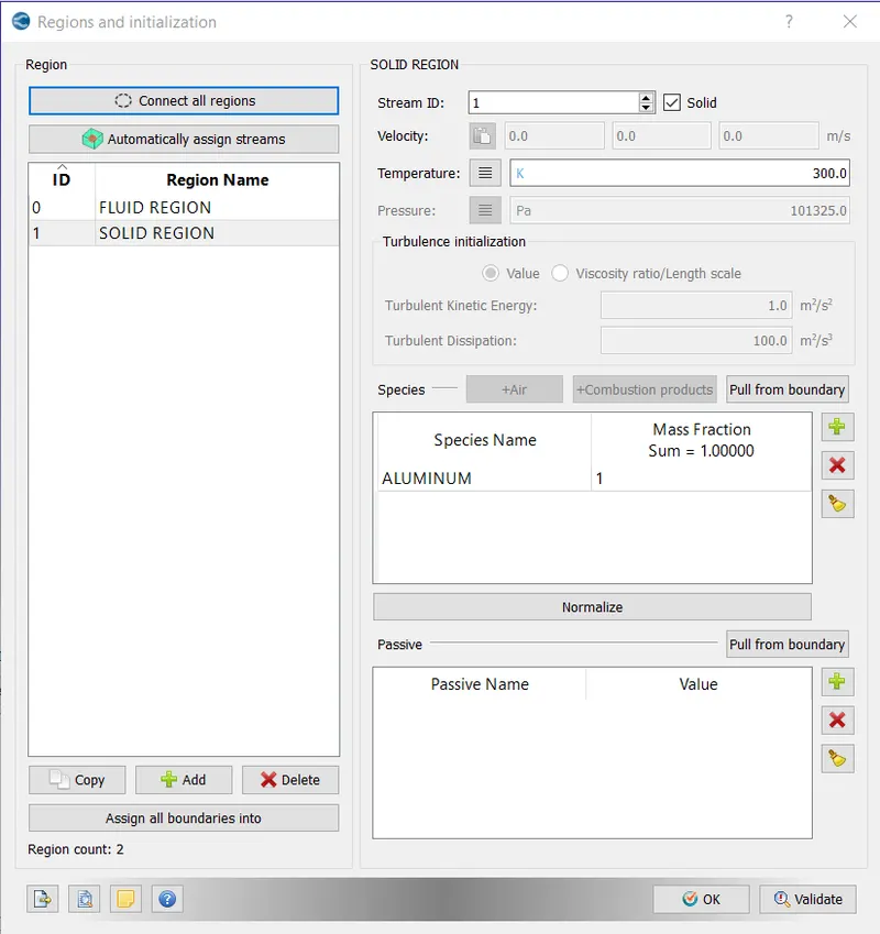
To configure the fluid and solid regions, case set up>Initial conditions>Regions and initializations.

To mark it as a solid, the solid box is checked. For fluids, the box need not be checled.

Streams:

• A stream is a collection of connected regions of the same phase(fluid,solid,etc)
• A converge solves for each stream independently , except the coupled interfaces.
• Each region must be assigned to a stream.

Converge creates the mesh for for each streamindependently. This allows for different embedding levels on either side of the interface .

Stram Id =0 for fluids

Stream Id =1 for static solids

Stream Id >1 for moving solids

6) Physical models:

Under the physical models, Turbulence models and the super cycling is turned on.

• Turbulence model:

Reynolds number is a dimensionless number that can be defined as the ratio of inertia force to viscous force.

Mathematically, `Re=(rho*V*D)/(mu)`

Where:

`rho`is the density of the fluid

`V`is the velocity of flow

`D`is the characteristic dimension of the cylinder.

Re = 7000

For flow through cylinders or pipe, Re>2900 accounts for fully developed turbulent flow.

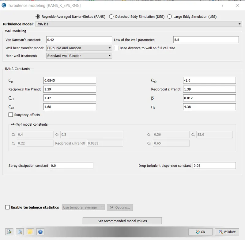
Turbulence model : RANS RNG K_epsilon

Other parameters are kept as provided by default by Converge studio.

• Super cycling:

Suoer Cycling is a method used by CONVERGE STUDIO in case of Conjugate heat transfer problems involving solid and fluid regions.

Fluid equations and solid equations are solved by two solvers separately. The fluid solver solves the equation much faster than the solid solver or the fluid equations converge much faster . This is basically due to the time scale difference for heat transfer in fluids and solids. This is where Supercycling comes into existence. What supercycling does is that the solver for the fluid domain pauses , till the solid equation converges. This period of pausing can be set manually called intervals.

1. Begin storing supercycle data: The initial time at which supercycle data starts storing data. this can be set to anything from zero to the simulation end time.
2. Solid side heat transfer solver: Can be steady or transient, independent of the solver used in run parametrs.
3. Time length for each cycle stage: This acclunts for the time interval at which the fluid solver is paused and solid solver is solved for.
4. Conduction CFL number , Relaxation factors are used to accelarate the solution.

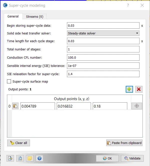
Time length for each cycle stage is manipulated from 0.01 to 0.03 and studied.

7)Grid Control:

• Base grid:

dx=0.004,dy=0.004,dz=0.004

Grid independence test is run for subsequent grid sizes, dx=0.003,dy=0.003,dz=0.003 meters and dx=0.002,dy=0.002,dz=0.002 meters.

8) Post processing parameters:

• Post variable selection : y+ file is selected from the combustion/turbulence section and included into the input files.

Results:

• Line plots:

1. Total cells :

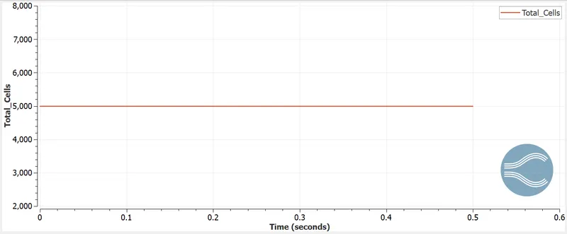
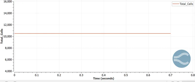
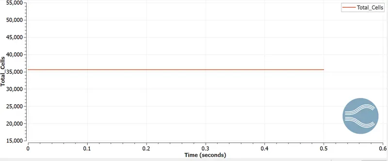
Grid size	Total number of cells
0.004	5000
0.003	10500
0.002	35000

2. Solid mean temperature:

Comparisons are done between three grid sizes ; 0.002 meters,0.003 meters and 0.004 meters.

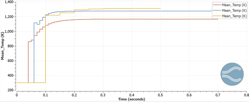
With the grid size decreases, the accuracy increases. Moreover the results converges faster.

Comparison between different supercycling intervals for the grid size 0.002 meters:

• Supercycle stream1 temperature:

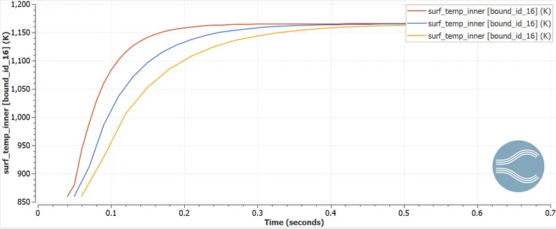
With increase in intervals the simulation time decreases

With increase in intervals, the number of iterations required to reach the convergence also incereses.

• Fluid mean temperature:

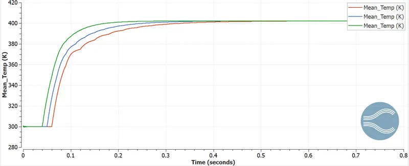
With Increase in the intervals, the number of iterations required to reach convergence is more

With increase in temperature the simulation time decreases.

• Solid mean temperature:

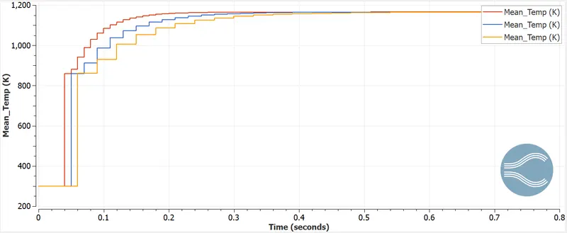
With Increase in the intervals, the number of iterations required to reach convergence is more

With increase in temperature the simulation time decreases

Post processing in paraview:

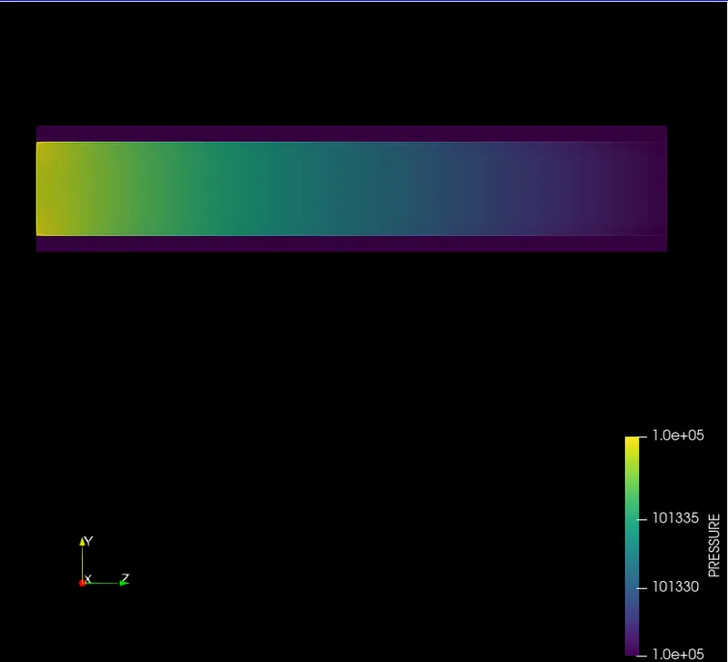
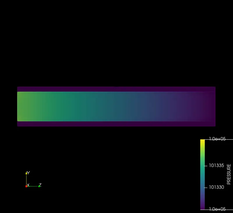
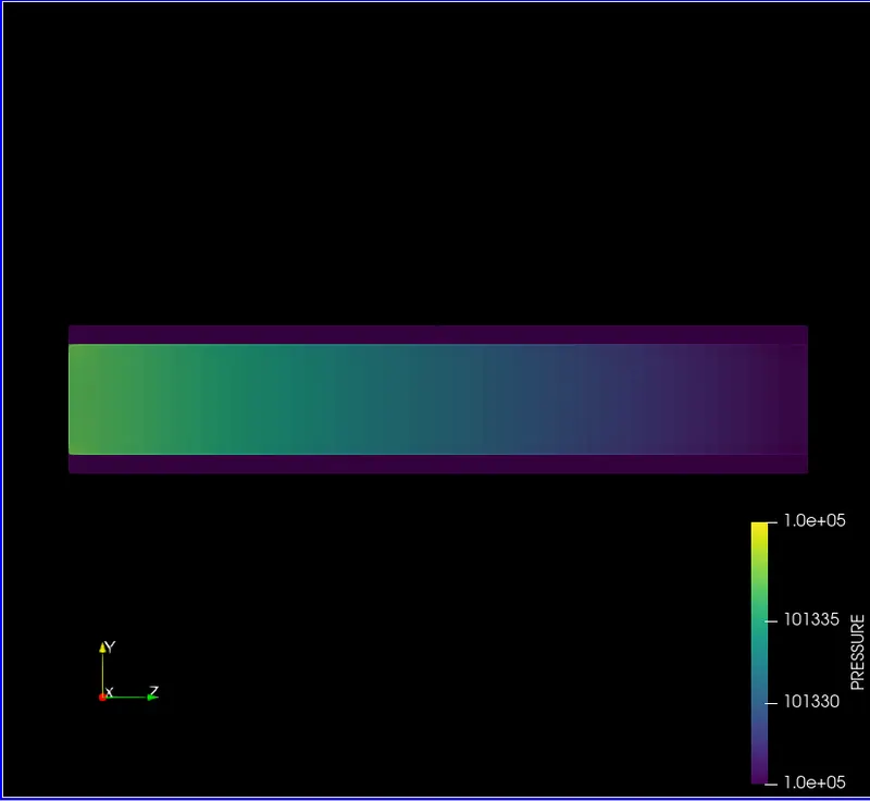
• Mesh generation: 1) 0.002 meters,2)0.003 meters3)0.004 meters

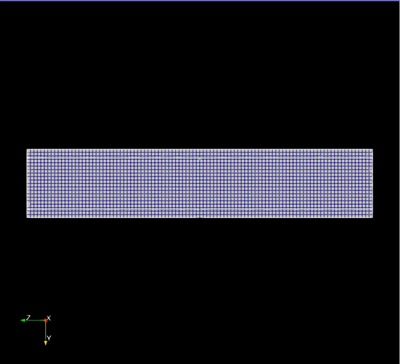
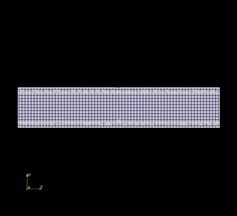
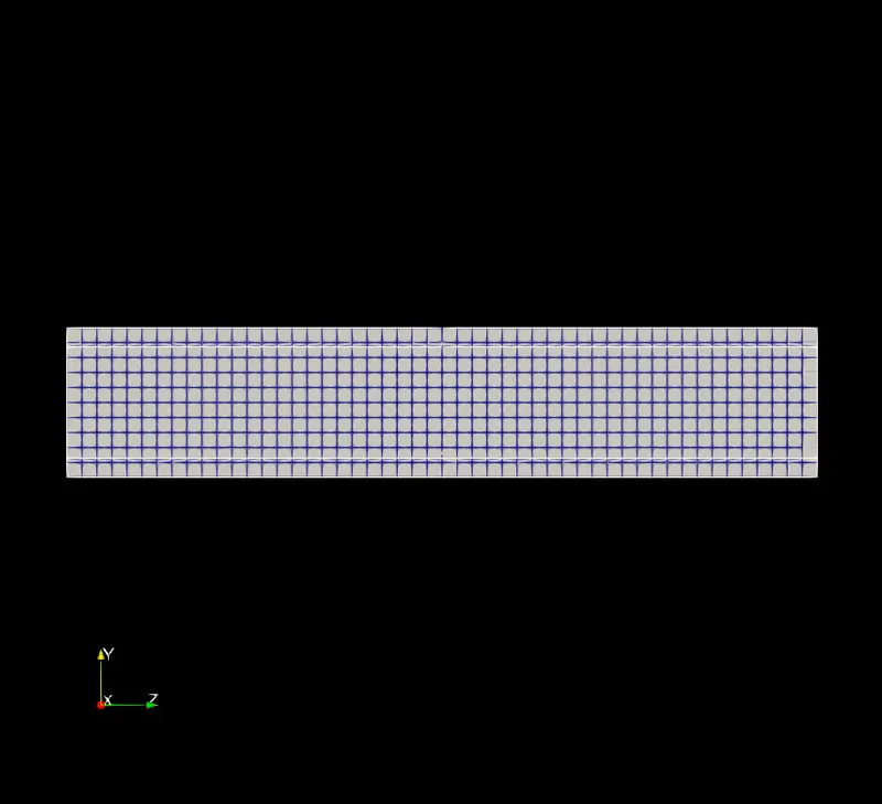
The geometry is cut along the x plane. Surface with edges option helps in visualizing the grid.

• temperature contour:

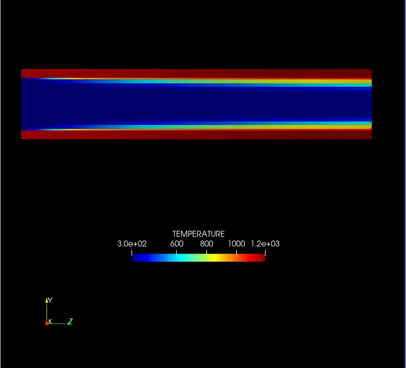
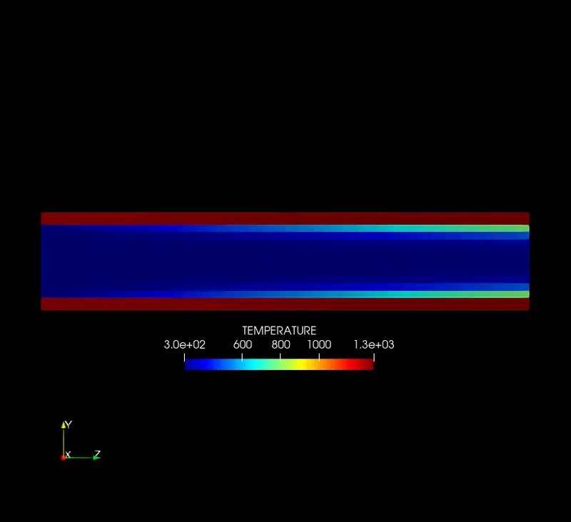
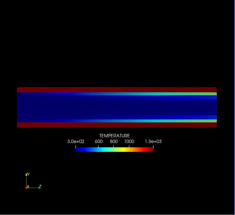
• Pressure contour:

• Y+ contour:

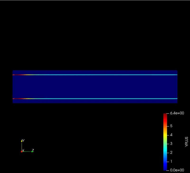
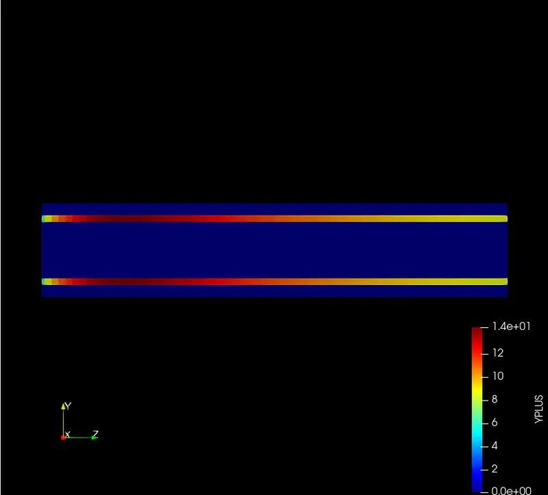
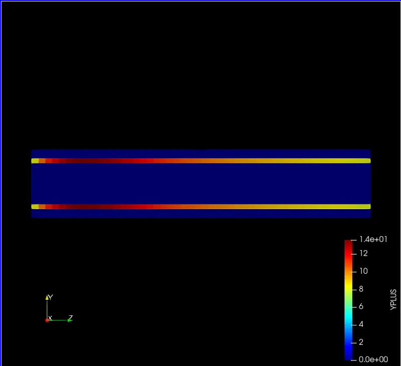
Y+ value ranges from 0 to 6.4 for grid size 0.002 meters.

Y+ value ranges from 0 to 14 for grid size 0.004 meters and 0.003 meters.

The animation of the simulation is provided through this link: https://youtu.be/JsZWEIEt51o

Conclusion:

• CHT analysis over a cylinder is done.
• The Y+ value is maintained and provided as an input file .
• The effect of different supercycle stage interval over the simulation convergence and the simulation time is studied.
• Mean temperature in Solid and Fluid zones is studied.