Week 6: Conjugate Heat Transfer Simulation
Introduction
In modern world the term ‘‘heat transfer’’ is very important. Latest products and processes are being invented and implemented day by day. Almost all such latest technology developments involve energy interaction and heat transfer. The application field of heat transfer ranges from material processing to space vehicle design. It includes micro scale applications like electronic circuit cooling as well as macro scale applications such as design of thermal protection system for space vehicles, thermal insulation of nuclear reactor, turbine blade cooling, solar panel design etc. Hence the need of today is the design of effective heat transfer devices. The foremost important parameters, that are to be analysed for the successful design of any heat transfer devices are temperature, heat flux and heat transfer coefficient of the surfaces exposed to heating or cooling environment. However accurate calculation of convective heat transfer coefficient requires boundary condition consists of the coupling of solid and fluid fields. Such a boundary condition assumes that the heat convected in or out to or from the solid is absorbed from or rejected to the fluid passing over the solid surface. This situation is highly complex to analyse theoretically since the wall and freestream parameters vary time to time. So, analytical solution for the simplest case of this heat transfer problem necessitates lot of simplified assumptions. Conventionally the solution for the problem has been sought explicitly for fluid and solid. That means, the heat conduction in the solid is solved by assuming a constant or time dependent heat flux at solid boundary and the flow field is analysed with the assumption of either constant wall heat flux or isothermal wall boundary. However, the isothermal wall (Tw = constant) boundary condition is far away from the reality in most of the practical heat transfer situations. Hence the heat transfer coefficient prediction employing isothermal boundary condition is also found to be erroneous. To have analytical or numerical prediction of heat transfer coefficient close to experimentally obtained values, one must focus on conjugating the boundary condition at the fluid–solid interface through coupled heat transfer analysis. Such a coupled field study is termed as Conjugate Heat Transfer (CHT)
CHT (Conjugate Heat Transfer)
However, it may be noted that Coupled field analysis is not just limited to CHT studies involving fluid and solid domains. Coupled field analysis or specifically CHT analysis is essential in a situation where solution domain consists of more than one sub-domain in which heat transfer is governed by different differential equations. In such a case suitable governing equations are to be solved in the respective sub-domains and these solutions need to be conjugated at the interfaces of sub-domains. Aforesaid explicit solution seeking and coupling are also inevitable even if the heat transfer is governed by same set of differential equations, but sub-domains are having dissimilar material properties. An ideal example of conjugate heat transfer situation is heat exchange between a solid surface with internal heat conduction and an external fluid flow passing over it, external tube of outer radius R0, which is heated to a constant wall temperature and rotates at constant angular velocity. A fluid field is kept between this rotating tube and an internal stationary hollow cylinder. The internal stationary cylinder is uniformly heated by a hot fluid flowing inside the stationary cylinder. Now a days CHT algorithms are widely employed for aerothermal design of gas turbine vanes due to better accuracy of this analysing technique. Heat exchanger design, development of thermal protection system for aerospace vehicles, heat treatment of metals and alloys etc. are some of the other important application fields where CHT studies have crucial role to play. Conjugate heat transfer problems can be solved by either analytical methods or by numerical methods. The analytical CHT studies require thorough understanding of the given heat transfer problem and involves complex mathematics. Such studies involve lot of simplifications based on certain valid assumptions. Hence the correctness of the solution depends largely on the validity of assumptions made. On the other hand, numerical CHT solution methods are relatively simpler if the numerical methods to be followed is clear. Moreover, a correctly implemented numerical CHT solver is not just limited to one CHT problem. Hence the same CHT algorithm can be applied to several CHT problems with minimum efforts in terms of solution domain modifications. The main governing equations considered for the conjugate heat transfer problems are: For steady or unsteady fluid flows: 1. Law of conservation of mass (The continuity equation) 2. Law of conservation of momentum (The Navier Stokes equations, 2D or 3D depending on the nature of f low) 3. Law of conservation of energy (The complete energy equation corresponding to dimensionality of the flow) Similarly for steady or unsteady conduction in the solid domain: 1. Two dimensional or three-dimensional unsteady energy equation Two- or three-dimensional steady Laplace or Poisson equations 3. One dimensional steady or unsteady conduction equation upon considering prevented or negligible heat conduction in other dimensions as in case of heat conduction through thin plates the selection of equation in the solid domain is based on the nature of heat conduction and that decides the solution strategy to be adapted in the solid domain. For instance, selection of one-dimensional heat conduction equation for the solid domain provides the ease of having simple analytical solution at the solid–fluid interface. However, the consideration of multi-dimensional heat conduction necessitates modelling and meshing of complete solid domain and solution seeking in it either using finite difference or finite element method. There are mainly two different methods of conjugating the solid and fluid domain solutions. The first method is a direct approach in which the complete set of equations is solved in both the domains simultaneously. The second method is the iterative approach where the fluid and solid domains are solved separately and only their solutions are conjugated at the interface. Elaborated details of these two methods, their relative merits and demerits are discussed in the subsequent sections. Conjugate heat transfer studies are superior to conventional heat transfer analysis since the simultaneous monitoring of changes in fluid flow and conduction-based heat transfer in solid are possible in CHT technique. In CHT analysis simultaneous solution of flow field of the fluid and temperature field of solid are carried out. The temperature and heat flux are exchanged at fluid–solid interface at every time steps. Hence real-time prediction of heat transfer rate and wall temperature is possible through such an efficient technique. The key task involved in any CHT solver development is formulation of proper communication strategy between fluid and solid domain. Such a bilateral information exchange is termed as coupling and the strategies followed for the same are known as coupling techniques. Since the invention of modern computers coupled field or Conjugate heat transfer studies have greatly overtaken conventional heat transfer analysis. There are large number of industrial heat transfer problems which require the CHT analysis. Analytical CHT studies have been presented by many researchers in the past. The phase of analytical heat transfer studies has been replaced by numerical CHT studies in the last two decades. The momentously increased speed and memory capacity of modern computers made the strategies of numerical solution seeking for governing equations of conjugate heat transfer problems simpler and faster. Thus to give a complete picture of evolution of CHT analysis, major computational studies in this area are reviewed in the subsequent sections followed by a brief summary of past analytical CHT studies.
Super-cycling
There are several challenges when solving the fluid and solid domains together. The largest challenge to overcome is the difference in time-scales associated with the heat transfer in the fluid and the solid. In general, heat transfer in the solid occurs more slowly than the convective and diffusive time-scales of the fluid. This disparity in time-scales is problematic for CFD simulations because simulations of long physical time periods can be computationally expensive. CONVERGE offers an alternative approach called super-cycling for overcoming the time-scale disparity. In super-cycling, the fluid solver is frozen periodically while the heat transfer in the solid is allowed to progress to steady-state. CONVERGE solves the fluid and solid phases in the same simulation without requiring you to stop and restart the simulation. Super-cycling significantly reduces the computational cost of the CHT simulation
Case-setup:
Calculation:
Reynolds number ( )=7000

 -Density in Kg/m^3-1.184 at 25 degrees Celsius
 -Velocity in m/s
L-Characteristic Length in m- 0.03 m
 -Dynamic viscosity in Kg/ms-0.00001837 Kg/m-s
 =3.62
=3.62 
Explanation:
-Model has been created in the Converge studio
(i)Geometry->create->cylinder is selected and provided a input as the radius for the cylinder
similarly created the solid part over the fluid domain
(ii)Deleted the front and the back faces with the help of delete tab under the repair option
(iii)Create->triangle to patch the deleted faces (solid surface normal to the flow)
(iv)Repair->patch is selected to create the inlet and outlet faces.
-creating the names for the boundary
(v)In this part, Surfaces of the CAD Model is assigned with the names by the name of boundary flagging.
Boundary->flag->add option is selected to create the necessary number of flags.
Selected the surfaces and click apply.

(vi) Normal Toggle On it is used to check whether the normals pointing towards the domain.if not, then transform->normal propagate change from the single face and select the one triangle that has the normal pointing opposite to the fluid domain and click apply.
-Solver Part
(vii)Application type-Time-Based simulation
(viii)Materials -predefined mixture as air, enabled gas, solid simulation
(ix)Solid is modelled is aluminium.
(x)N2, O2 is added under the species
(xi)Solver type - Transient
(xii)Simulation carried out for 1 seconds
(xiii)PISO Scheme is used, and density-based solver is utilised.
(xiv)Inlet-5 m/s, outlet pressure -101325 Pa, Heat flux on the outer solid wall is -10000 W/m^3.
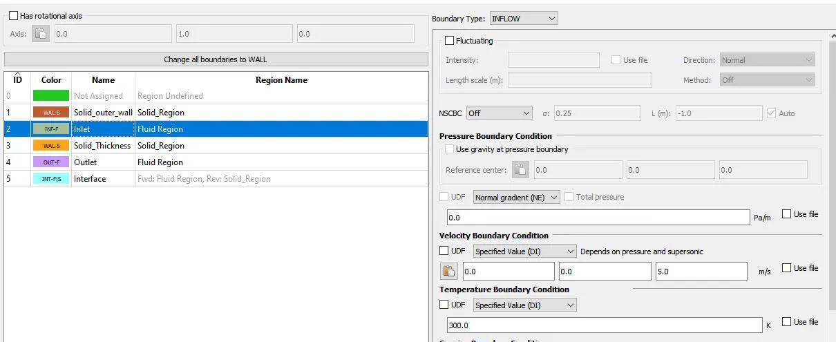


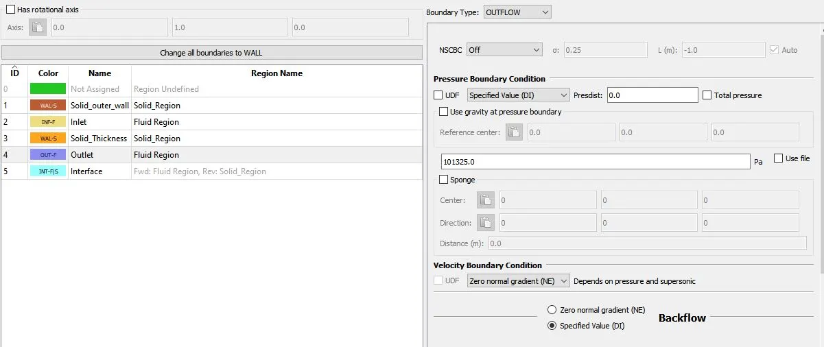

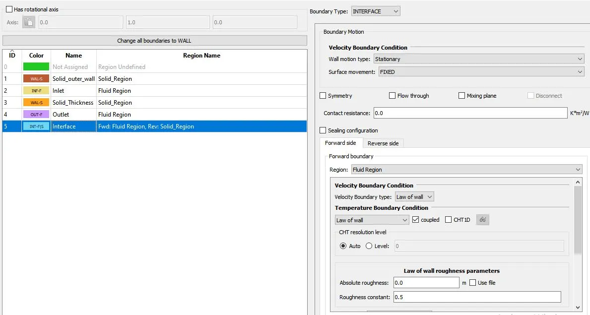
(xv) Create the regions and provided the input values for initialisation and then regions will be assigned to the wall Boundary conditions.
(xvi)k-e RNG turbulence model is used.
(xvii)Super cycle modeling is used.Steady state solver will be assigned for the thermal part and created the monitor points.
(xviii) add needed parameters for post processing
(xix)open cygwin and navigate the case setup folder.
(xx) Ran the simulation by typing the command "mpiexec -n 2 converge --license explore" in cygwin terminal.
Grid dependence test:
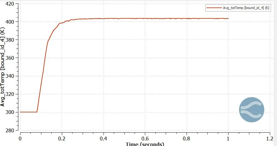
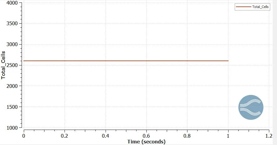
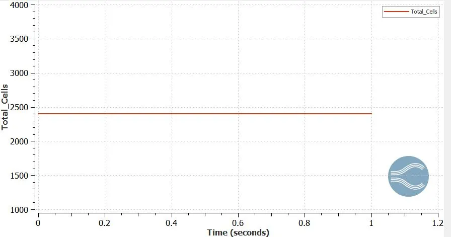
Supercycle stage interval-0.03 is used to carry out the grid dependence test with different mesh sizes. They are 5.4 mm, 4 mm, 2 mm grid sizes.
Plots:
Fine Grid-2 mm
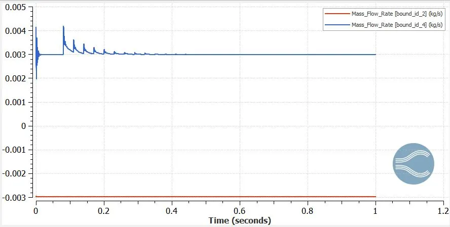
Fluid Region
Solid Region
Medium Grid-4 mm
Fluid Region
solid region
Base Grid-5.4 mm
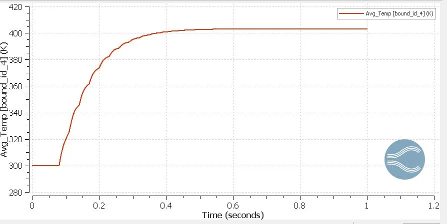
Fluid region
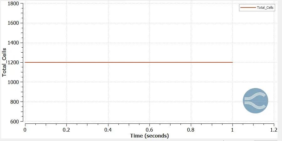
Solid region
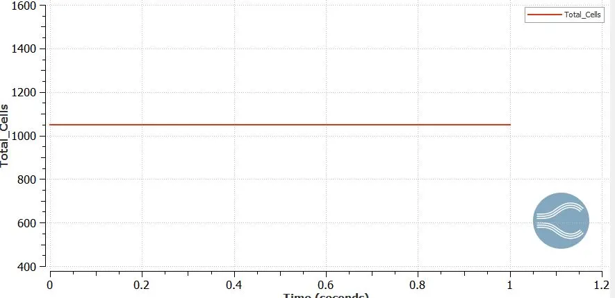
Supercycle stage interval:
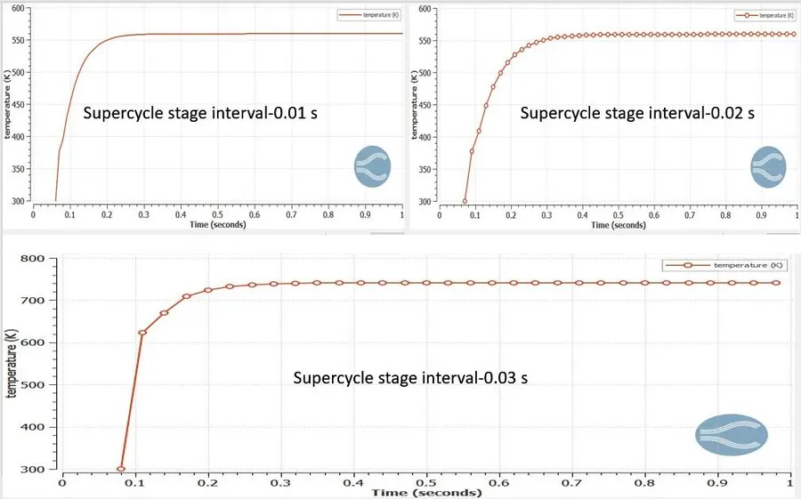
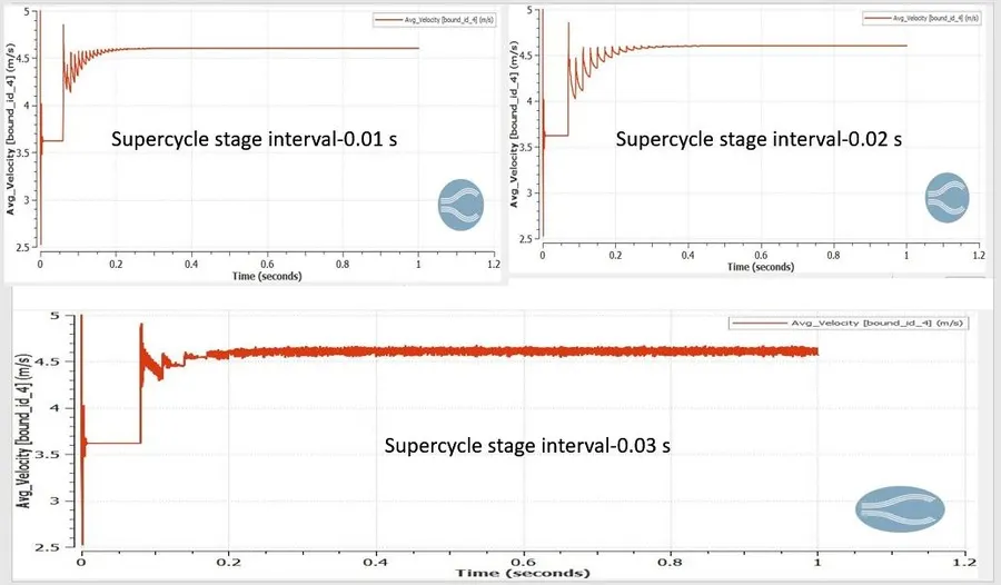
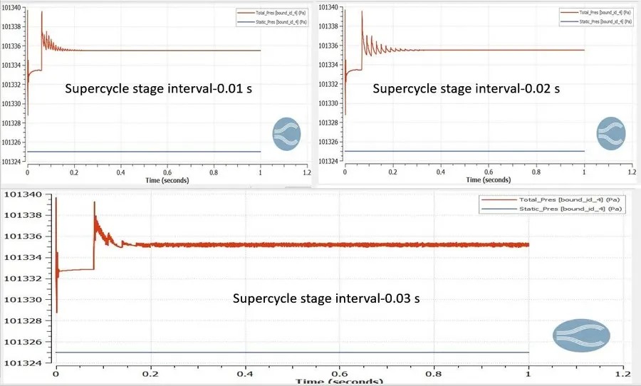
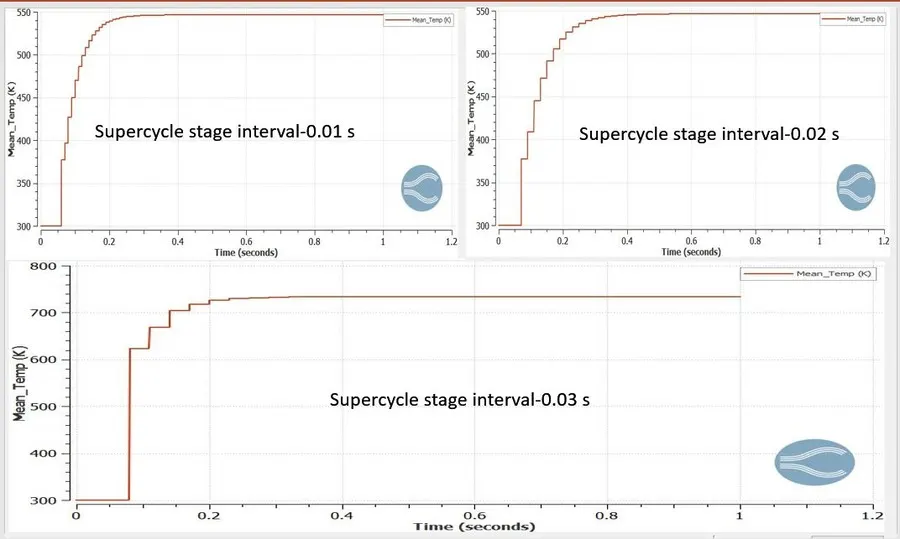
The simulation performed by varying the supercycle stage time interval as 0.01,0.02,0.03
Plots:
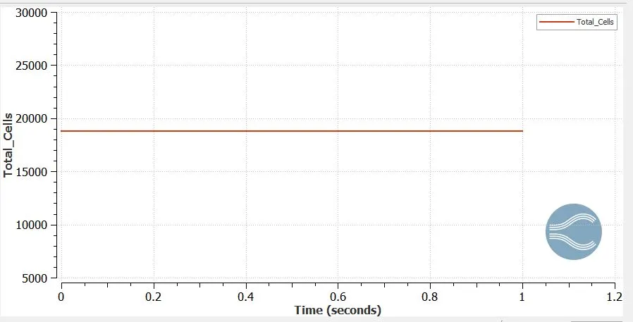
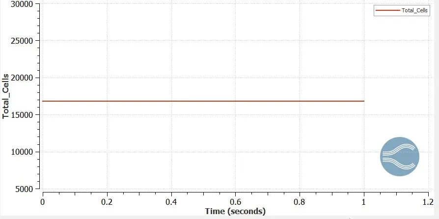
Load Balance
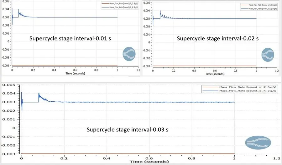
Monitor Plot
Conclusion:
| Grid_size in m | Cell Count | outlet Temperature in K |
| 0.0054 | 2250 | 403.2 |
| 0.004 | 5000 | 403.2 |
| 0.002 | 35600 | 409.4 |
-We can see that fine grid outlet temperature changed is less than 5% then it can be concluded as grid independently values are getting.
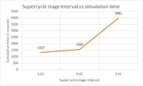
-As the supercycle stage interval increasing with the simulation solving time
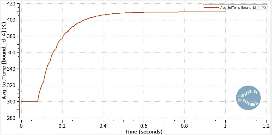
-We can observe the difference in the temperature at the outlet of the fluid for varying in supercycle stage interval. As the 0.01, 0.02 s supercycle stage interval will have nearly same fluid outlet temperature when compared to the 0.03 s case.
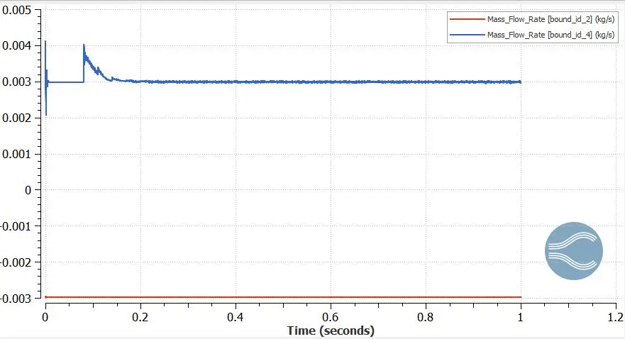
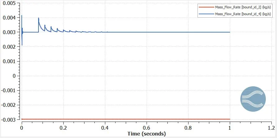
-In the range of 0-0.1 s. velocity and pressure gets fluctuated due to effect of temperature. Heat flux is defined at the walls might be the reason for varying temperature.
-Velocity at the outlet is increased due to temperature increase. Convection and conduction heat transfer increased the temperature on the fluid.