Week 6: Conjugate Heat Transfer Simulation

AIM:

• To simulate a flow through a pipe with air as the flow fluid and post process the results.

OBJECTIVE:

• grid dependency test
• y+
• Effect of supercycling

INTRODUCTION AND THEORY:

"Heat transfer" is known as the flow of thermal energy from one region to another region occupied by any matter (solids and fluids) where the rate of heat transfer is proportional to the temperature difference between the regions/matter. “Conjugate heat transfer” (CHT) is used to describe the variation of temperature between the solids and fluids due to the exchange of thermal energy between them.

Modes of heat transfer

• Heat Transfer in a Solid - Conduction: Diffusion of heat due to temperature gradients in solids. A measure of the amount of conduction for a given gradient is heat conductivity. Conduction is described by Fourier’s law defining the conductive heat flux, q, proportional to the temperature gradient

q = -k∇T

For a time-dependent problem, the temperature field in an immobile solid verifies the following form of the heat equation:

`rhoc_p (delT)/(delt) = grad.(kgradT) + Q`

• Heat Transfer in a Fluid - Convection: When heat is carried away by moving fluid. The flow can either be caused by external influences, forced convection or by buoyancy forces, natural convection.

Due to the fluid motion, there are three contributions to the heat transfer:

1. Convective contribution:Depending on the properties of the fluid and its region of flow, the domination of conduction and convection varies.
2. Viscous effects:Due to the fluid flow, the viscosity creates heat. This effect is often neglected due to its negligible value but should be taken into account for high-velocity cases.
3. Density effects:When the density becomes related to the temperature, the domain will have different densities at different locations based on the temperature distribution. This variation in density can cause the compression which in-turn generates the heat.

In addition to conduction due to these contributions, the transient heat equation for the temperature field in a fluid:

`rhoc_p(delT)/(delt) +rhoc_pu.gradT = alpha_pT((delP_A)/(delT) + u.gradP_A) + tuo : S +grad.(kgradT) +Q)`

• Heat transfer due to Radiation: Transfer of energy by electromagnetic waves between surfaces with different temperatures, separated by a medium that is at least partially transparent to the (infrared) radiation. Radiation is especially important at high temperatures, e.g. during combustion processes, but can also have a measurable effect at room temperatures.

SUPERCYCLING:

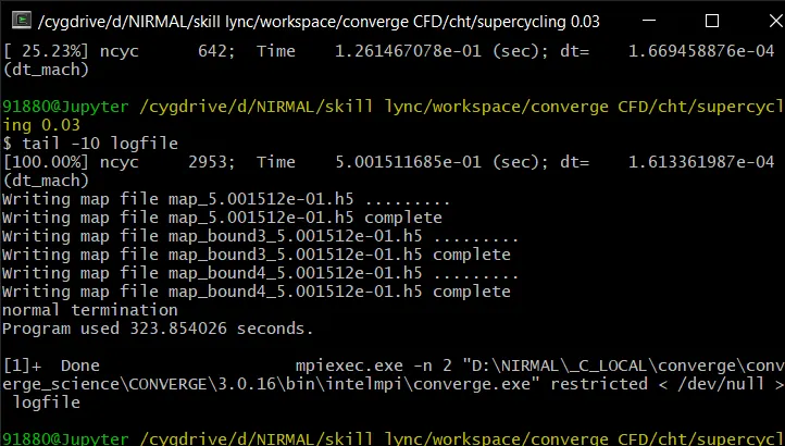
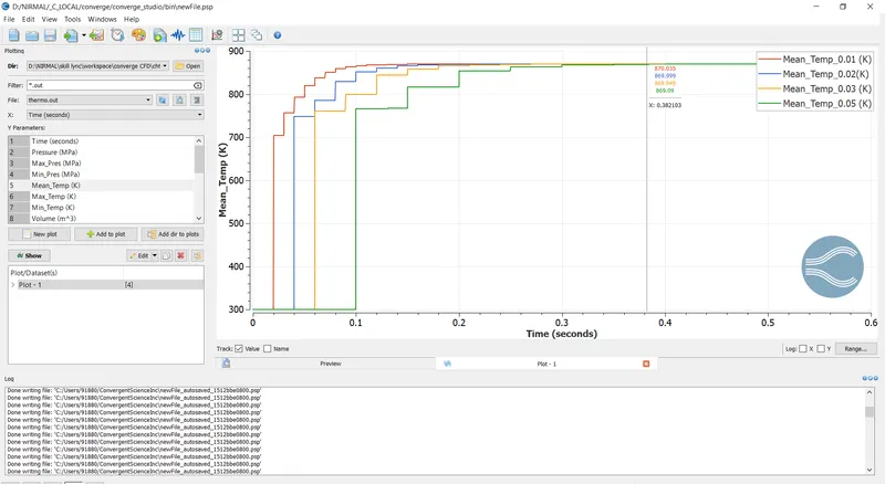
Super-cycling is a method used by CONVERGE Studio in the case of conjugate heat transfer problems with a solid and liquid regions. The integral problem here is that both solvers cannot run at the same speed since solving in the fluid domain is much faster owing to the time scale difference for heat transfer in liquids as compared to solids. This causes problems during the solution given that the solid side solver would not have reached a steady state/convergence in the time the liquid solver does. This is where the concept of super-cycling can be used. The basic idea of super-cycling is that the solver for the fluid domain is paused until the solver for the solid domain converges. This pausing is done in intervals that can be set by the user.

Y+:

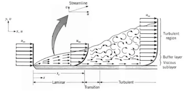
The image attached shows the boundary layer development. We first start in the laminar region, then transition to the turbulent region. Near the wall, due to the viscous forces, the velocity is dragged to zero and as the boundary layer develops, the velocity will reach free-stream velocity. This is termed as the no-slip condition.

We can use the no-slip condition if we know the flow is completely laminar. This would mean that we are resolving the flow in the laminar region whatever the grid size. This, however, doesn’t hold if the flow is turbulent. Turbulent flows have a smaller laminar region near the wall and if we are to resolve the gradients at such a small region, we’d need a very small grid size.

This is where the y+ value comes handy. The y+ value is a non-dimensional term that can be used to understand how coarse or fine our grid is. This can then be used to determine if wall functions need to be used or not. From the image attached above, we need to either be in the viscous sub-layer or the turbulent region.

If we were in the viscous sub-layer, that would mean a y+ of less than 10 and if we were in the turbulent region, it would mean a y+ of greater than 30. This is very significant in our making the decision of using or not using a wall function.

Y+ = y*u_t/v

Where, y is the distance from the wall

u_t is frictional velocity

v is kinematic viscosity

SIGNIFICANCE:

The y+ value denotes wherein the y+ vs u+ curve we are with respect to the cell size. It is undesirable to have a cell size that leads to a y+ of between 10 to 30 since the modelling of flows transitioning from laminar to turbulent is not easy and is still being researched.

Due to this fact, it is better to have a y+ of less than 10 meaning we'd be at the laminar region or have a y+ of greater than 30 where we can go with a wall function and still achieve results. The y+ value can be used as a marker based on which we can decide on the base grid size and make a decision based on the computing power as to whether the grid needs to be refined further or coarsened.

GEOMETRY SETUP:

• GEOMETRY CREATION:

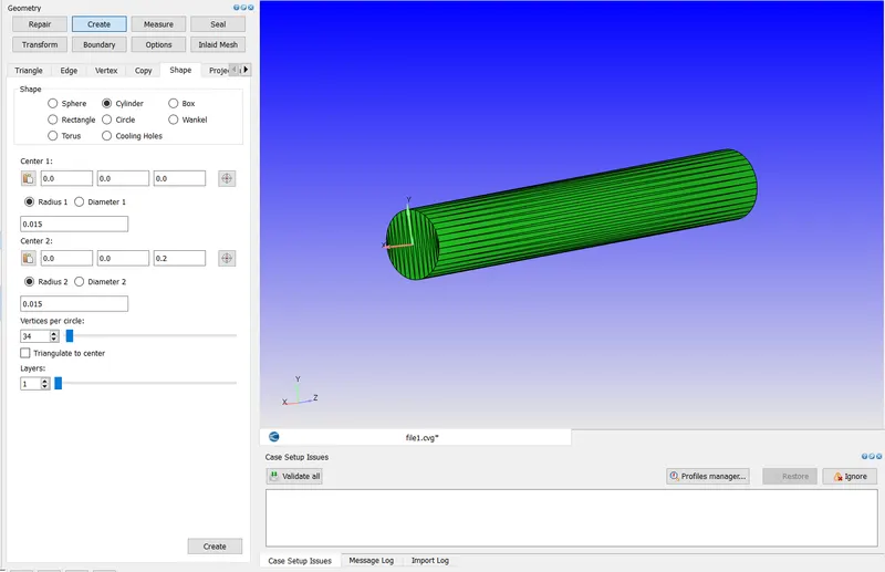
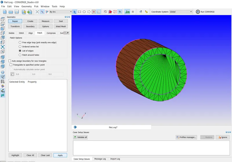
Geometry is created by going to create > shape > cylinder.

First inner cylinder of 0.015 m radius of 0.2 m length is created.

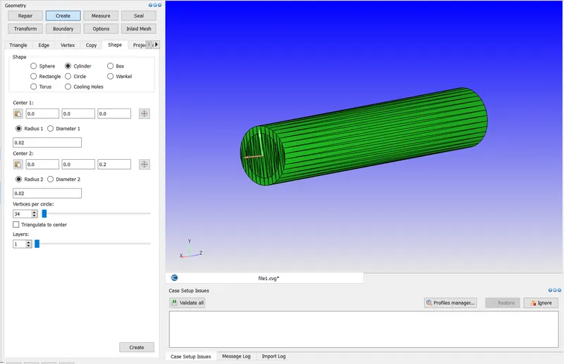
Then outer cylinder of 0.020 m radius of outer cylinder of 0.20 m length is created.

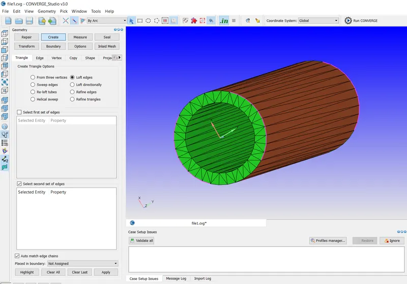
The sides of cylinders are deleted and patched by using patch tab in geometry.

• NORMAL ORIENTATION:

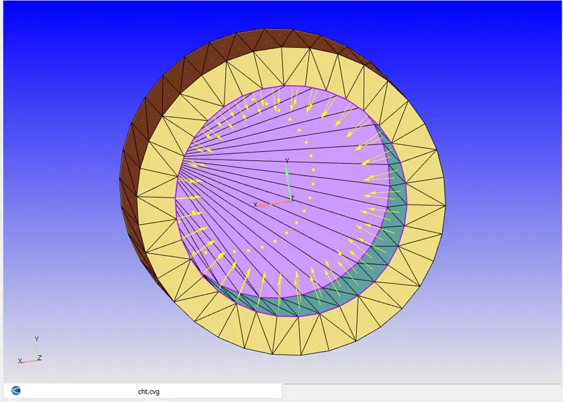
Normal are changed such that it points inwards.

• CREATING BOUNDARIES:

The boundary are created for the geometry under boundary flag tab.

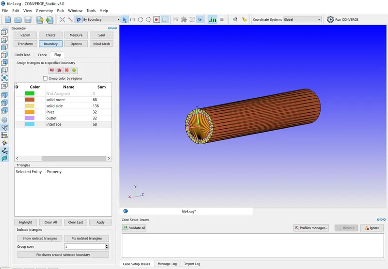
The boundaries are assigned to the faces and the name of the boundaries are edited and click apply.

• DIAGNOSIS:

The diagnosis is runed and checked for problems for the geometry.

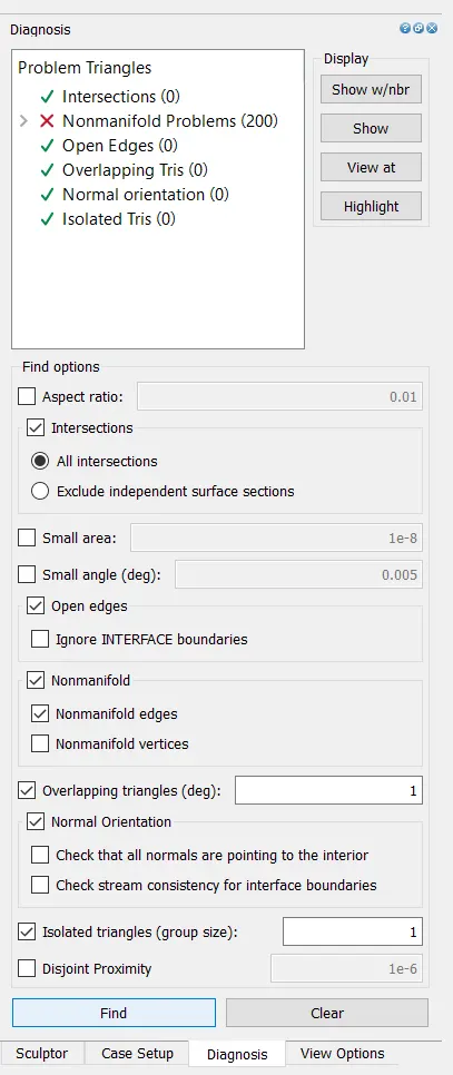
The non manifold problem will exist but it is ok for conjugate heat transfer problem

BEGIN CASE SETUP:

• APPLICATION TYPE:

On the right panel go to the case setup tab, select begin case setup.

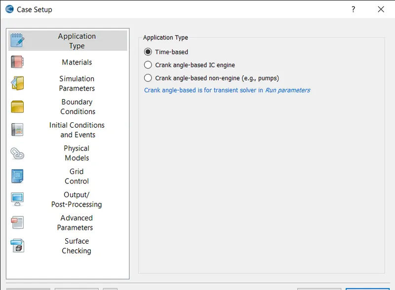
Select the application type as time-based and select apply and done.

• MATERIALS:

Select materials and unselect the checkbox reaction mechanism and select species and then select the predefined mixture as air then click apply and done.

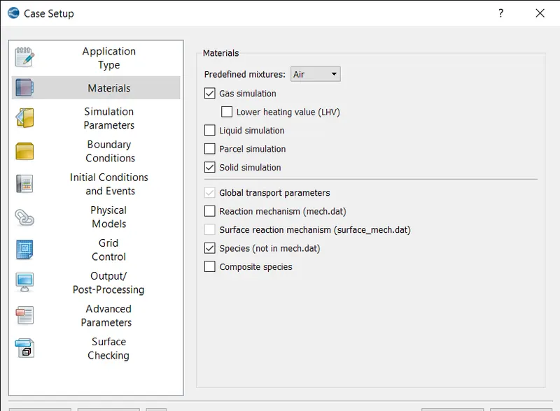
• GAS SIMULATION:

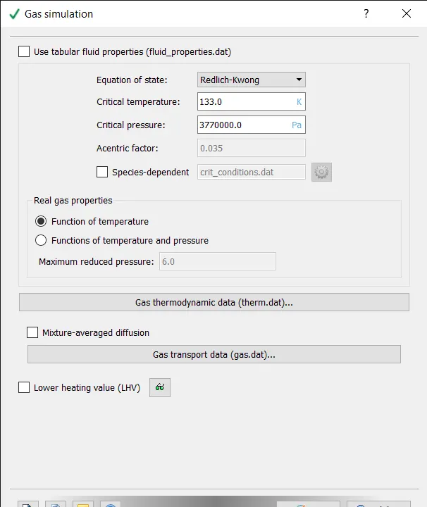
The default values are selected and press ok.

• SOLID SIMULATION:

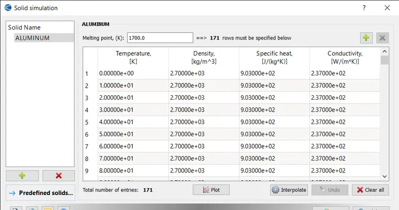
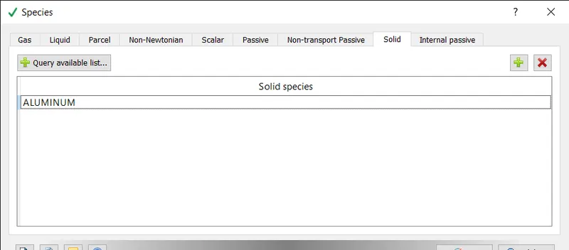
Under predefined solids add aluminium to the solid simulation step.

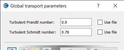
• GLOBAL TRANSPORT PROPERTIES:

Select global transport properties, keep the default values and press ok.

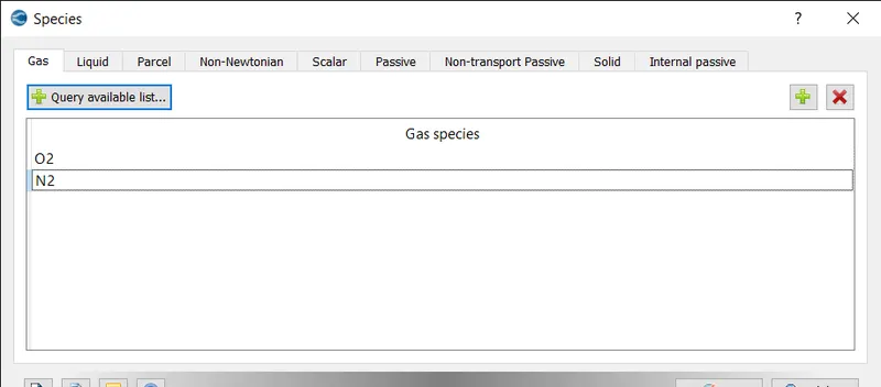
• SPECIES:

In gas tab add O2 and N2 as species

In solid tab add aluminium from query available list.

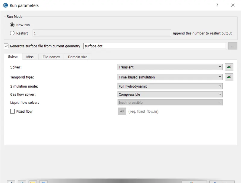
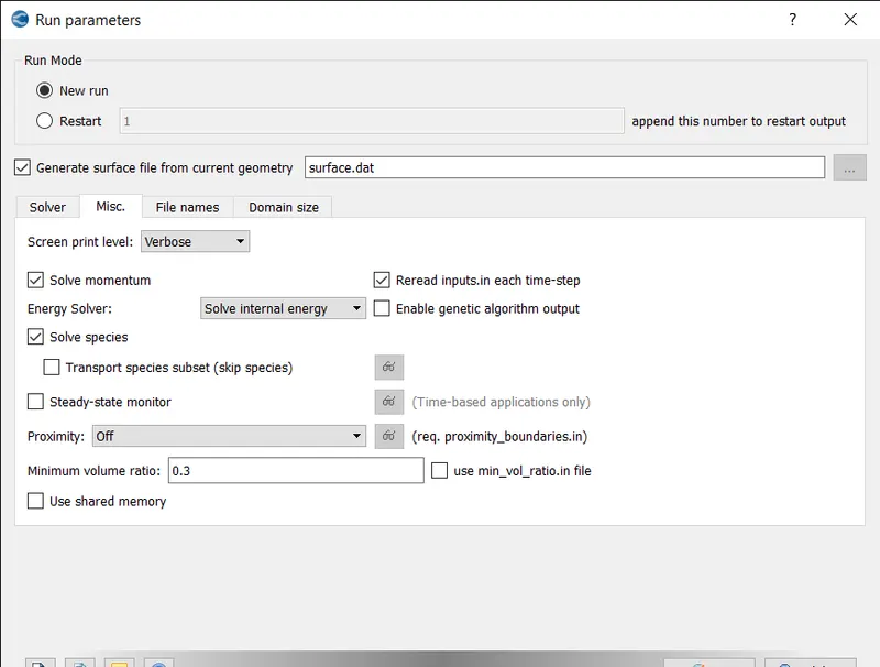
• RUN PARAMETERS:

Under solver tab select solver as transient solver.

• MISC TAB:

Under misc tab uncheck use shared memory option and click ok.

• SIMULATION TIME PARAMETERS:

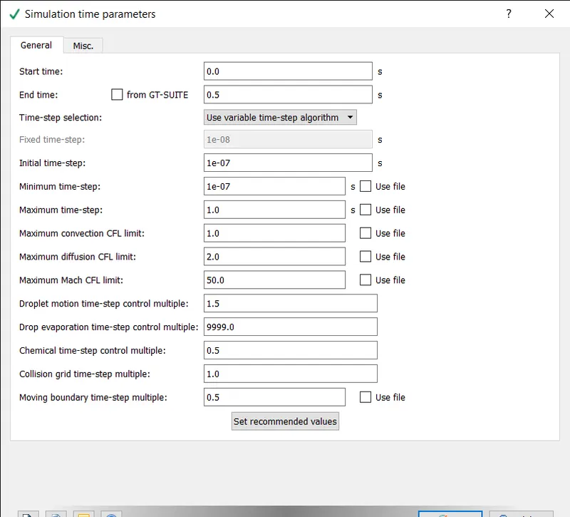
Set the start time, end time, initial, minimum and maximum time steps as shown above.

• SOLVER PARAMETERS:

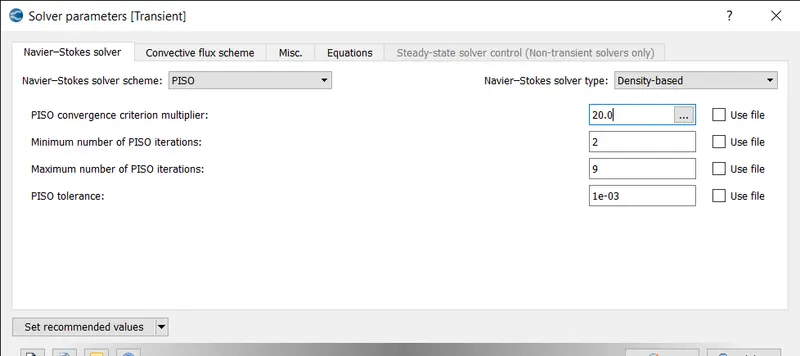
Select the Navier-stokes solver type as density based and click ok.

• REGIONS AND INITIALIZATIONS:

Fluid:

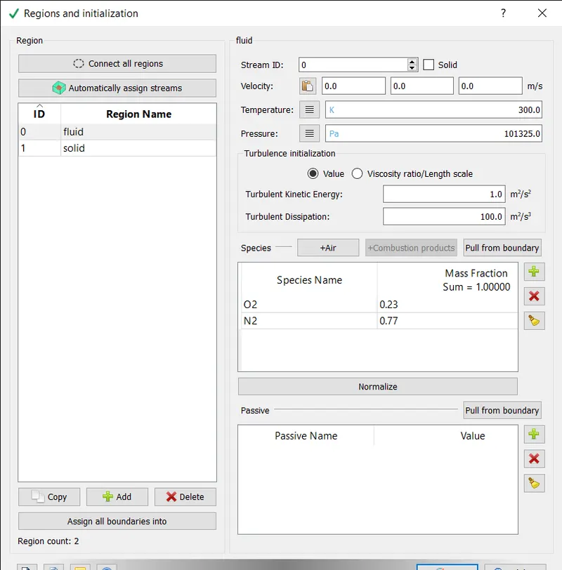
A fluid region is created and air is added as species.

Solid:

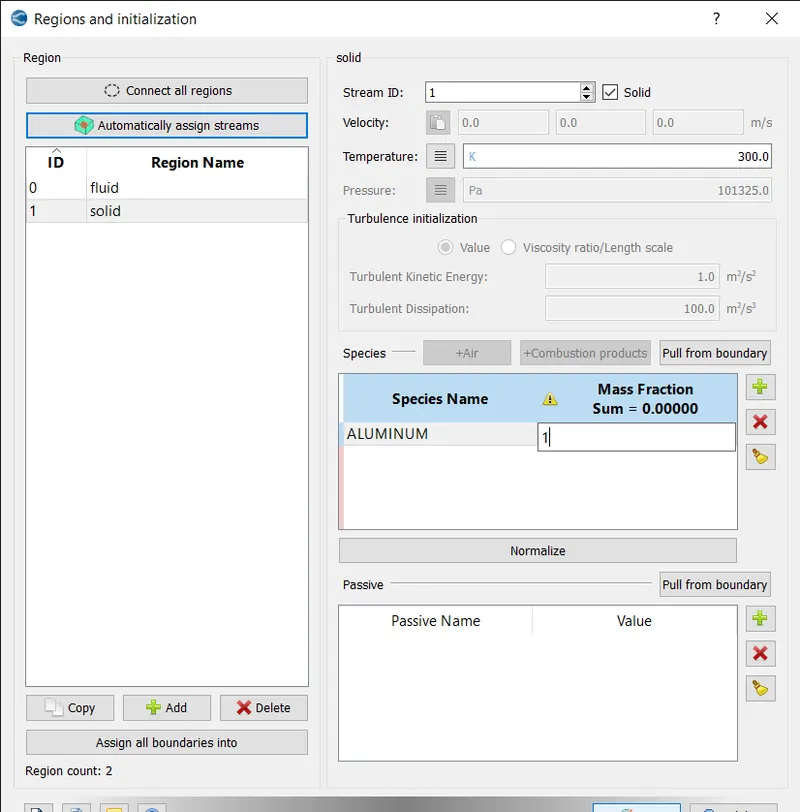
A solid region is created and stream id is set to 1 and solid box is checcked and aluminium is added as species and mass fraction is set to 1.

• BOUNDARY CONDITIONS:
• INLET:

Inlet velocity is calculated by using the below formula,

`Re = (rho*V*D)/(Dynamic. Viscosity)`

Taking Re as 7000 and diameter as 0.3m.

Then properties of air at 1 atm pressure at 15 c are

rho = 1.225 kg/m^3 and dynamic. viscosity = 1.802 * 10^-5 kg/m-s

7000 = 1.225*V*0.3/1.802*10^-5

V = 3.43m/s

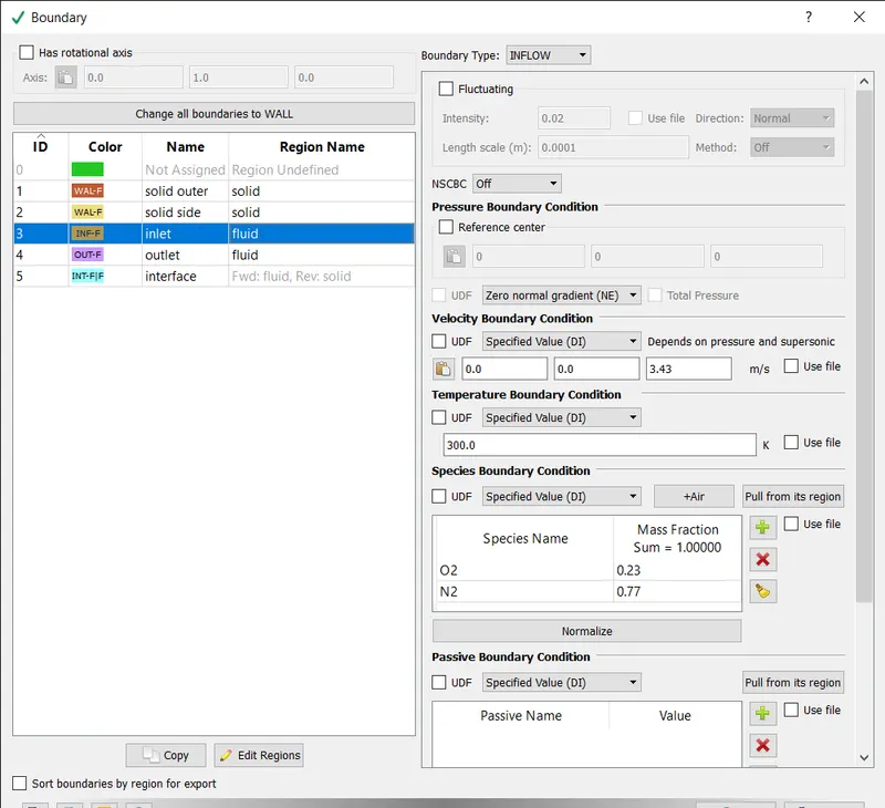
For inlet, set the pressure boundary condition as zero normal gradient and velocity as 3.43m/s in z direction and select air for species boundary conditions.

OUTLET:

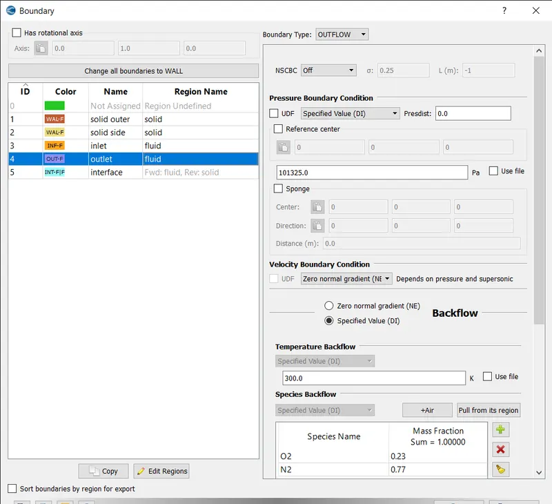
Set the outlet pressure boundary conditions as specified value of 101325 pa and for species backflow select air.

• SOLID OUTER:

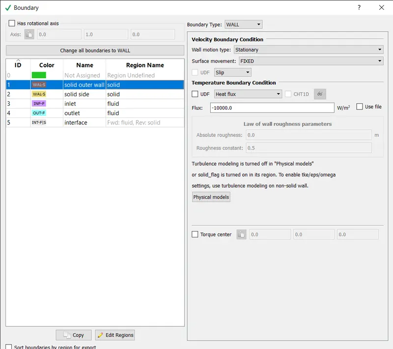
select boundary type as wall and velocity b.c as slip and temperature b.c as heat flux of -10000w/m^3.

• SOLID SIDE:

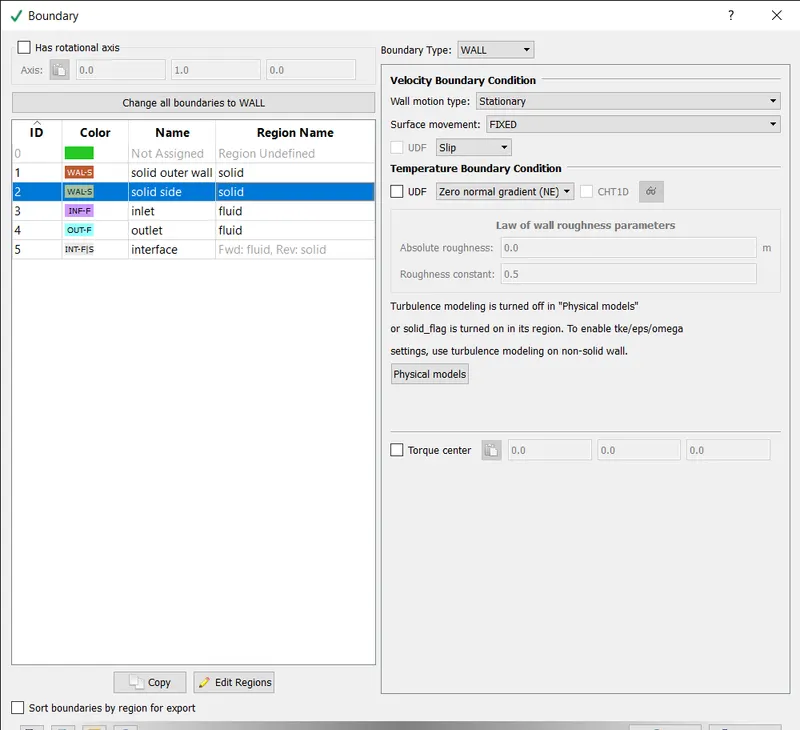
select the boundary type as wall and velocity b.c as slip and temperature b.c as zero normal gradient.

• INTERFACE:

FORWARD:

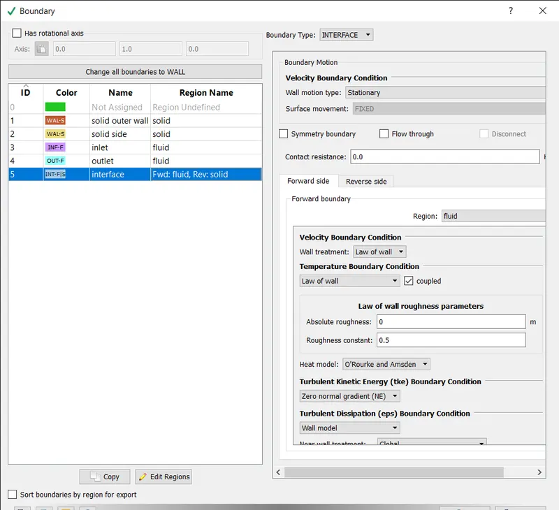
In forward side, select region as fluid and velocity and temperature b.c as law of wall.

REVERSE:

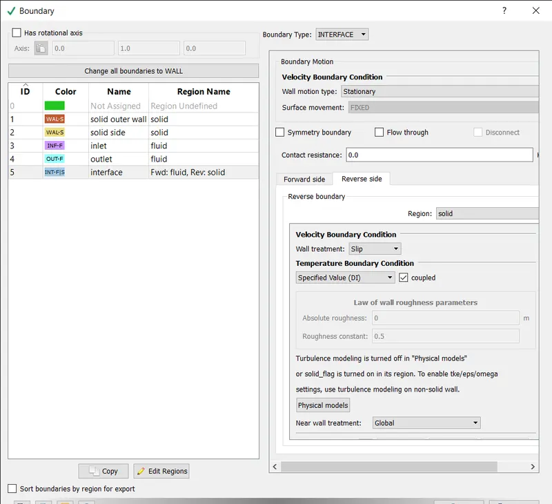
In reverse side, select region as solid and velocity and temperture b.c as slip and specified value respectively.

• PHYSICAL MODEL:

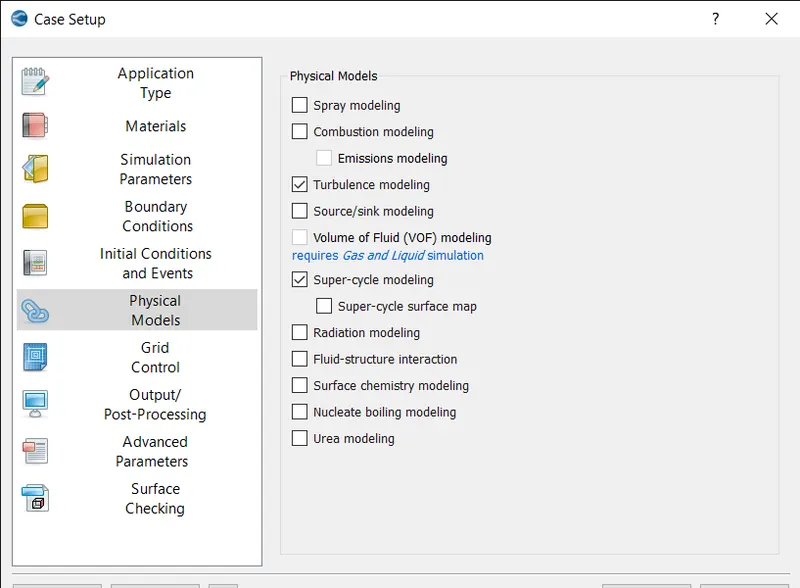
In physical model, the turbulence modelling and super-cycle modelling is check and clicked ok.

• TURBULENCE MODEL:

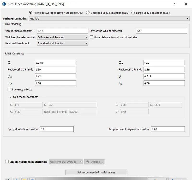
The RNG K-epsilon is selected for turbulence model and the values are kept default.

• SUPERCYCLING:

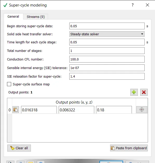
In supercycling the values are assigned as shown above and clicked ok.

• BASE GRID:

The base grids are defined as 0.004 m and press ok.

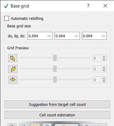
The base grid is changed for three different cases.

• POST VARIABLE SELECTION:

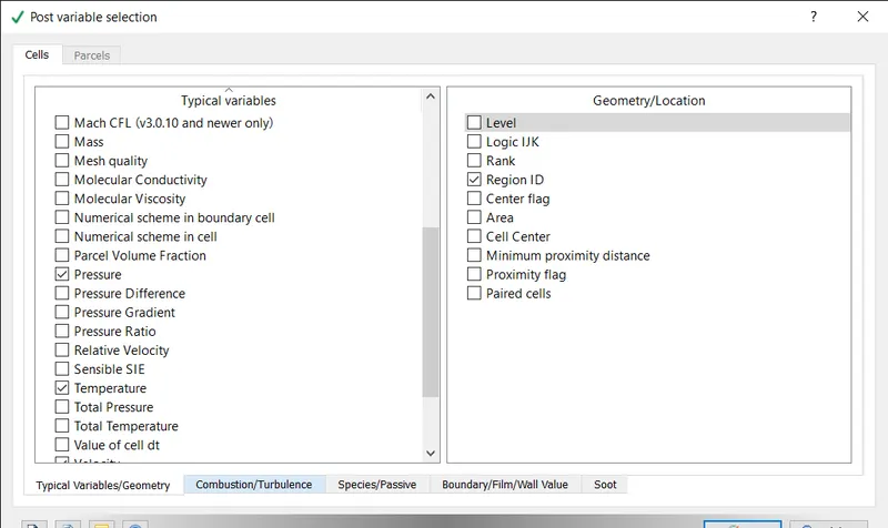
Keep the default values in typical variables tab.

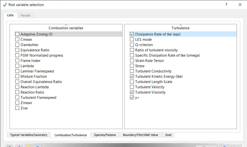
Under combustion/turbulence the Y+ is checked and others are kept default..

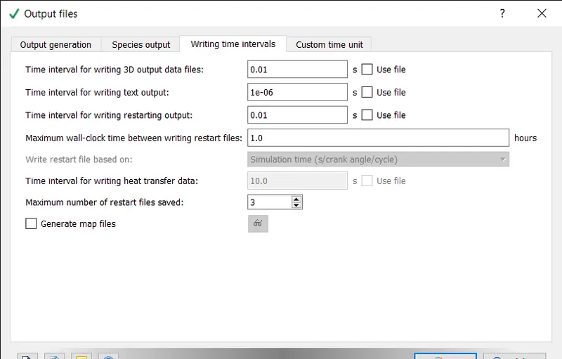
• OUTPUT FILES:

The interval for writing 3d output data files and restarting outputs are defined.

• Exporting the input files to a folder
• Then the executable is pasted inside the folder
• The simulation is run in Cygwin.
• The postconvert executable is pasted in the output folder.
• The post conversion is done on Cygwin and converted into the type that paraview reads.
• The results are then post processed using paraview.

RESULTS:

CASE 1: dx = dy = dz = 0.002 m

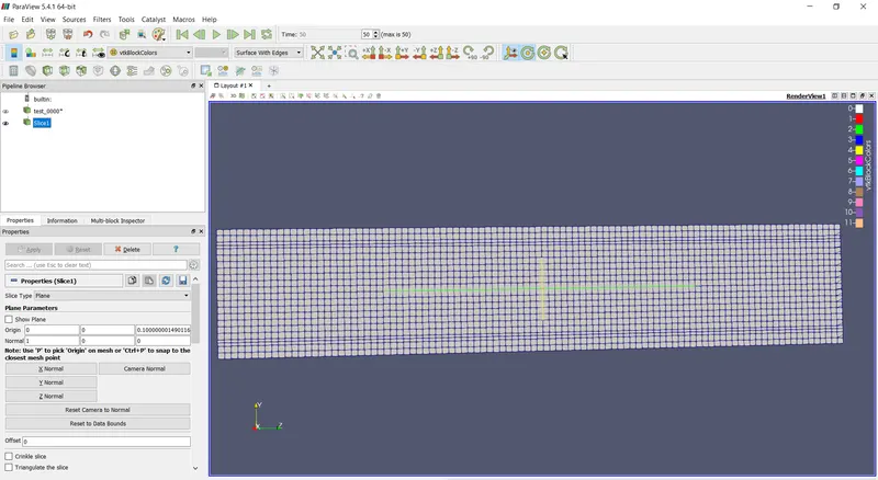
MESH:

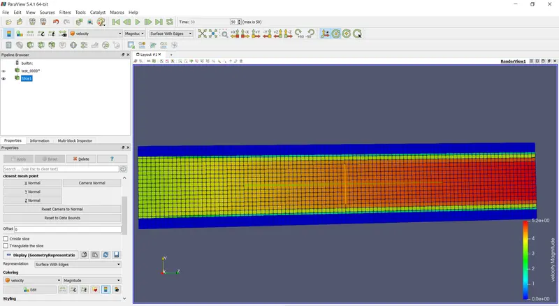
VELOCITY CONTOUR:

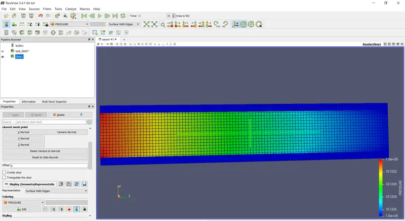
PRESSURE CONTOUR:

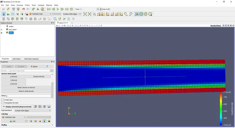
TEMPERATURE CONTOUR:

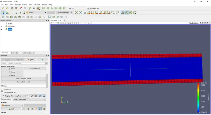
DENSITY CONTOUR:

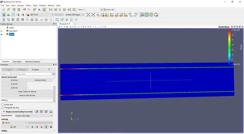
Y+:

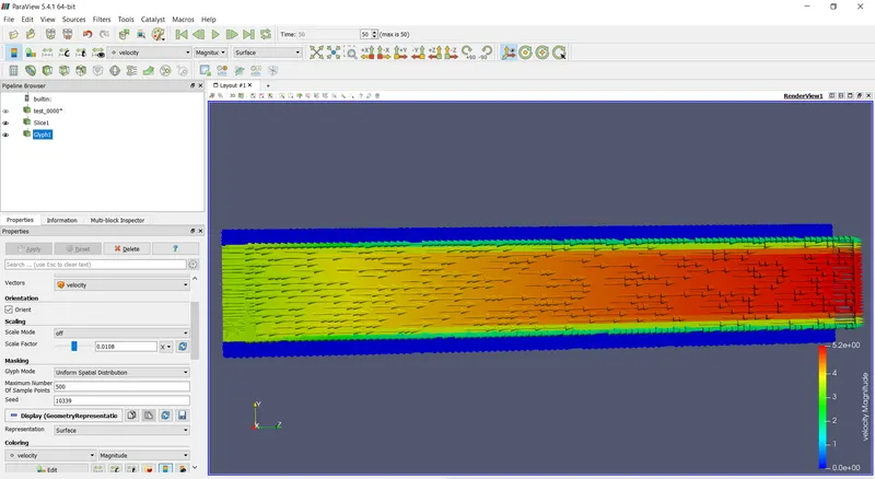
VELOCITY VECTOR:

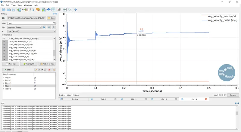
AVERAGE VELOCITY PROFILE:

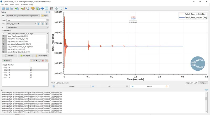
AVERAGE TOTAL PRESSURE PROFILE:

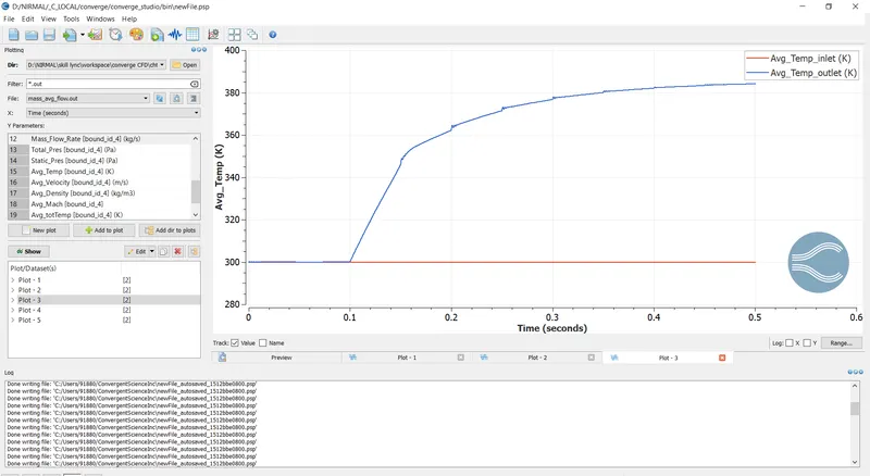
AVERAGE TEMPERATURE PROFILE:

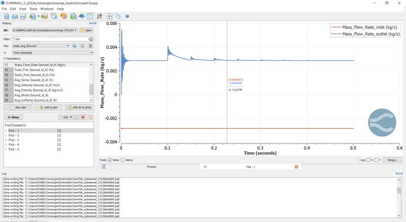
AVERAGE MASS FLOW RATE PROFILE:

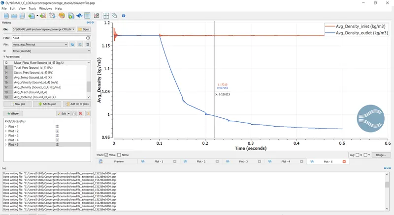
AVERAGE DENSITY PROFILE:

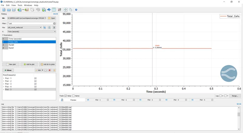
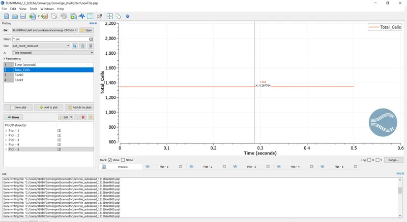
CELL COUNT:

VELOCITY ANIMATION:

https://drive.google.com/file/d/1ngmjyg3QgMn-z8GGk9bzo-HW2lwcZLW1/view?usp=sharing

CASE 2: dx = dy = dz = 0.004 m

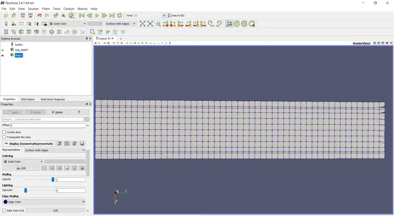
MESH:

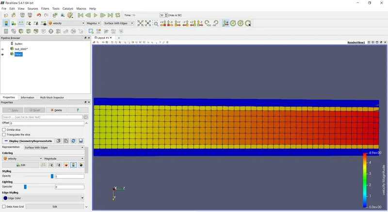
VELOCITY CONTOUR:

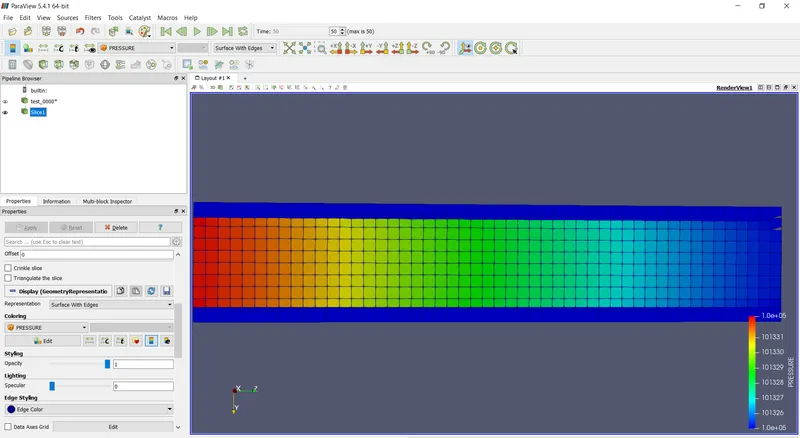
PRESSURE CONTOUR:

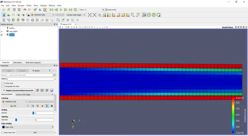
TEMPERATURE CONTOUR:

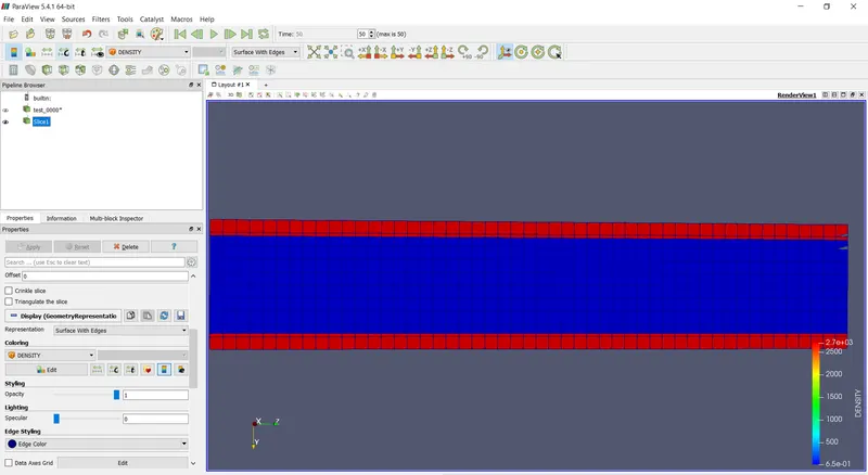
DENSITY CONTOUR:

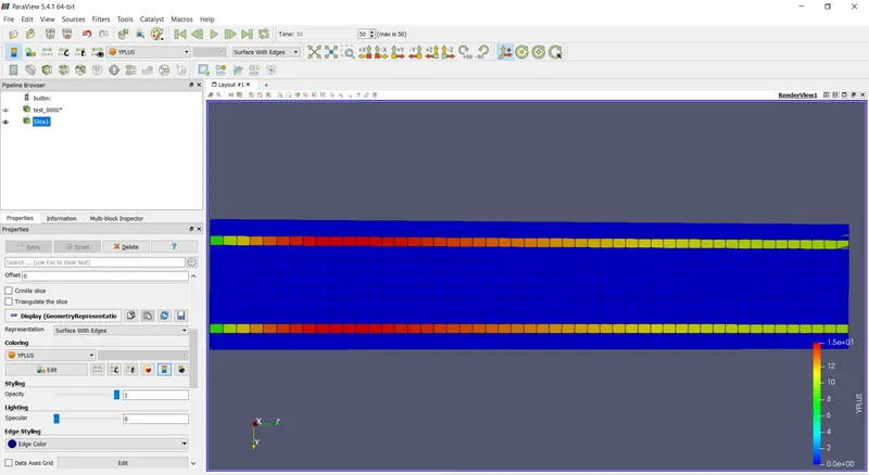
Y+:

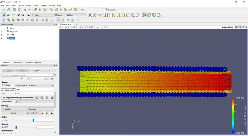
VELOCITY VECTOR:

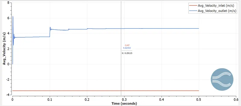
AVERAGE VELOCITY PROFILE:

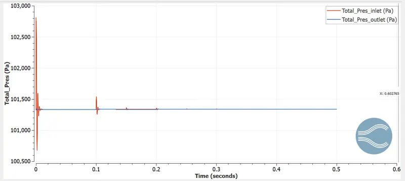
AVERAGE TOTAL PRESSURE PROFILE:

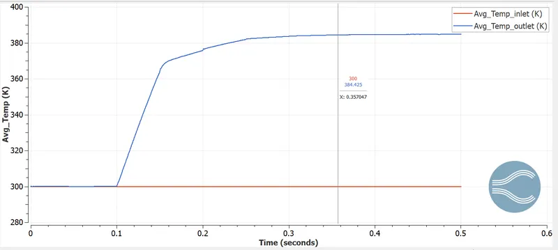
AVERAGE TEMPERATURE PROFILE:

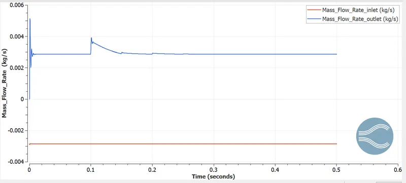
AVERAGE MASS FLOW RATE PROFILE:

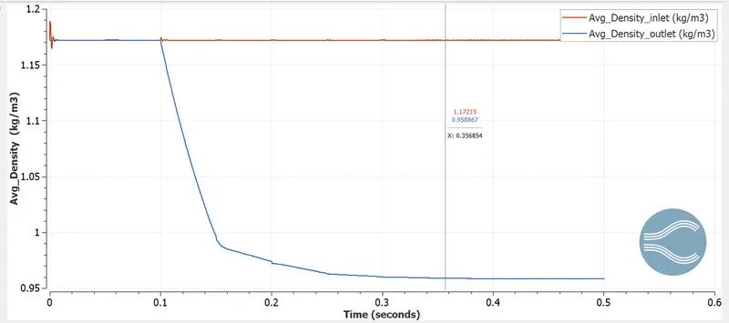
AVERAGE DENSITY PROFILE:

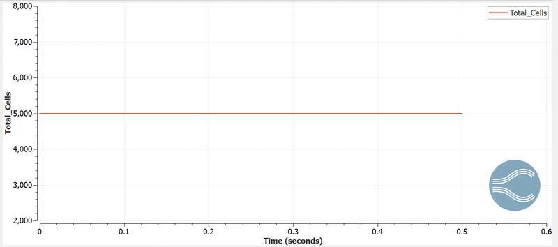
CELL COUNT:

VELOCITY ANIMATION:

https://drive.google.com/file/d/1CBmyac3kq3EOy2XfzjihMBClfR-Em72d/view?usp=sharing

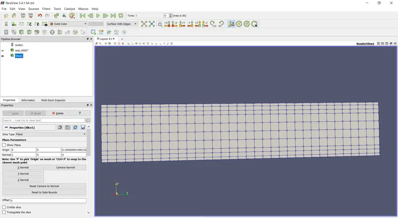
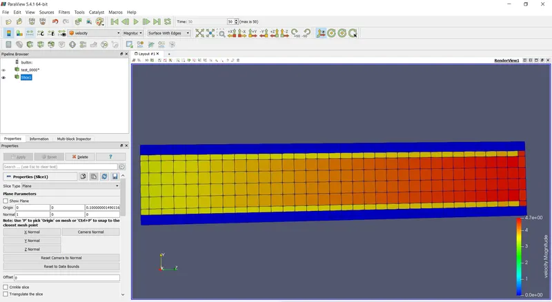
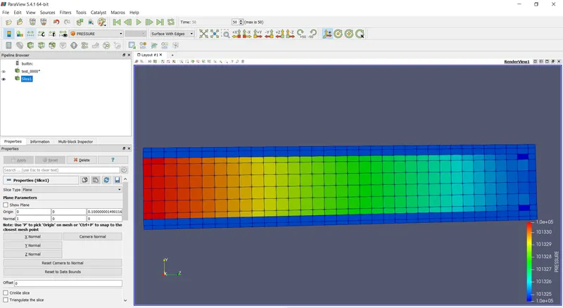
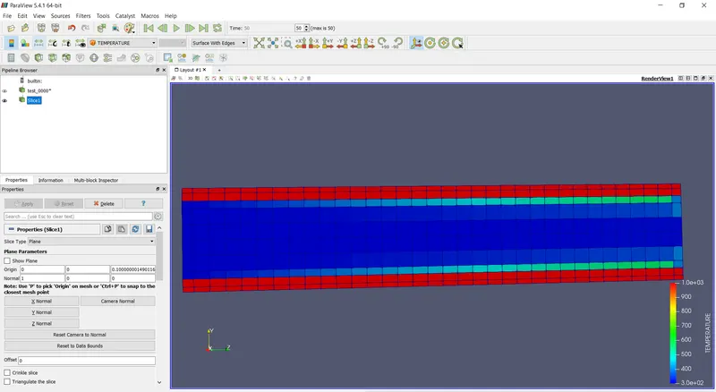
CASE 3: dx = dy = dz = 0.006 m

MESH:

VELOCITY CONTOUR:

PRESSURE CONTOUR:

TEMPERATURE CONTOUR:

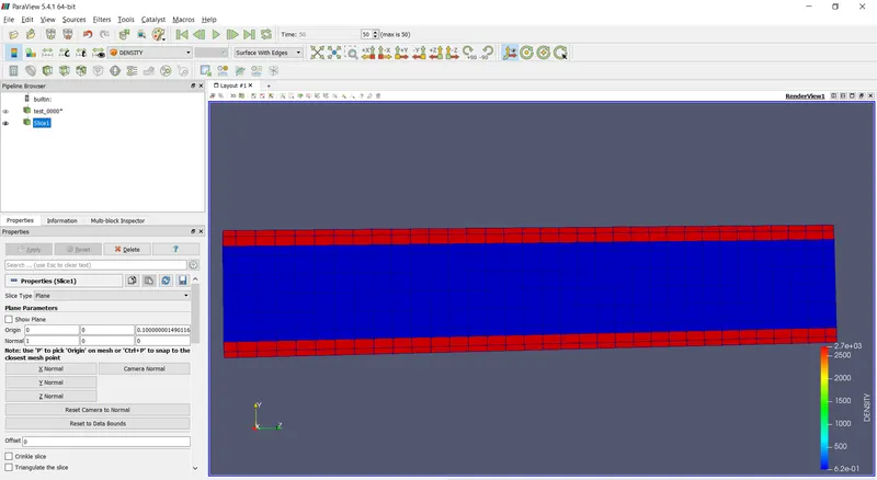
DENSITY CONTOUR:

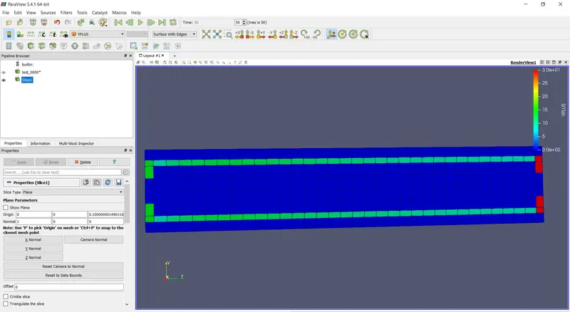
Y+:

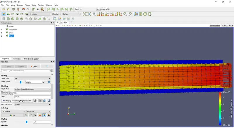
VELOCITY VECTOR:

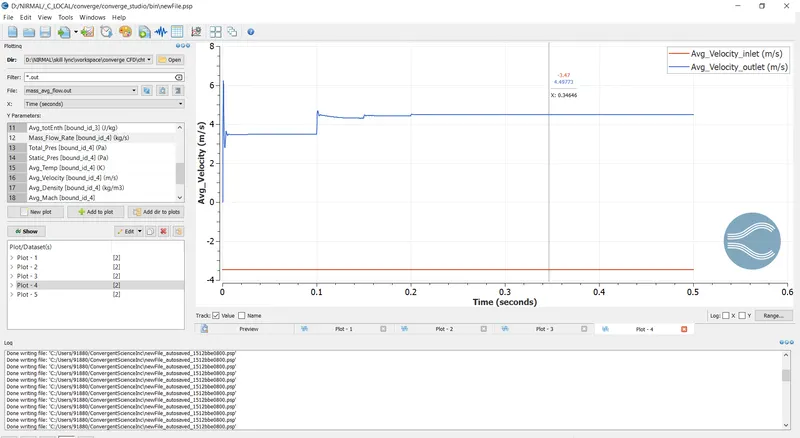
AVERAGE VELOCITY PROFILE:

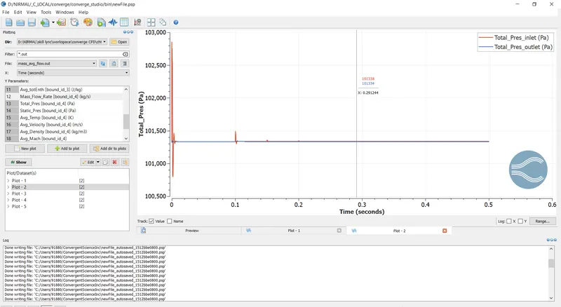
AVERAGE TOTAL PRESSURE PROFILE:

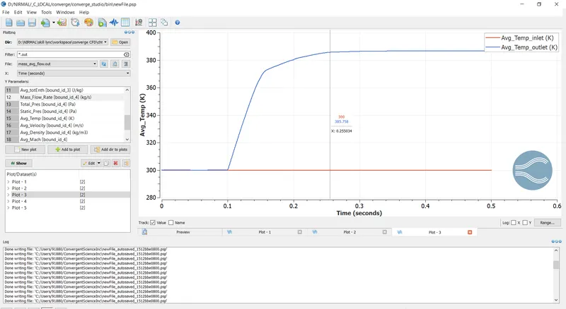
AVERAGE TEMPERATURE PROFILE:

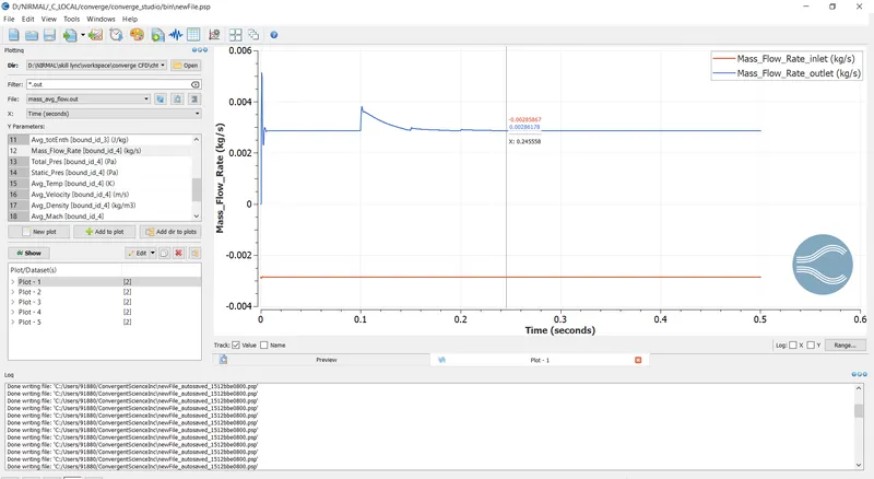
AVERAGE MASS FLOW RATE PROFILE:

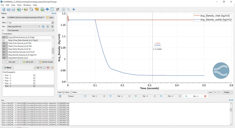
AVERAGE DENSITY PROFILE:

CELL COUNT:

VELOCITY ANIMATION:

https://drive.google.com/file/d/1Ak6XgHcGNE4Tp6v6-g8Gma5Zq9BSPtWJ/view?usp=sharing

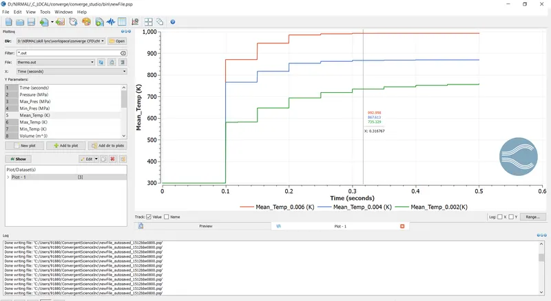
GRID DEPENDENCE TEST:

CONCLUSION:

• As the grid size decreases the time taken for simulation to converge increases.
• As mesh size decreases the solid region temperature decreases.
• As mesh size decreases the y+ value also decreases.
• Temperature contour shows that fluid temperature increases near the boundary as it is contact with pipe.
• Pressure contour shows that the presssure decreases from inlet to outlet as the flow propagates from high pressure to low pressure.

EFFECT OF SUPERCYCLING:

BASE MESH GRID - 0.004M:

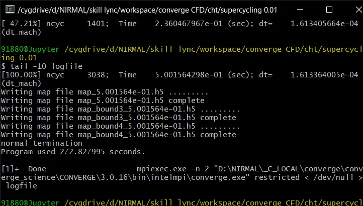
CASE1 0.01:

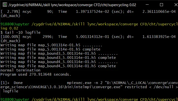
CASE2 0.02:

CASE3 0.03:

MEAN TEMPERATURE:

CONCLUSION:

• As the supercycling interval increases the simulation time taken to converge increases.
• The number of cycles taken to converge decreases as the supercycling interval increases.