Conjugate Heat Transfer Simulation through a pipe
AIM:
The aim of this project is to simulate conjugate heat transfer through a pipe.
OBJECTIVES OF THE PROJECT:
- Observe the mesh generation in ParaView.
- Observe the y+ value over the geometry
- Perform a grid dependence test
- Observe the effect of the supercycle stage interval on the simulation time.
- Create an animation of parameters varying through the geometry
THEORY:
What is Conjugate heat transfer?
Conjugate heat transfer corresponds with the combination of heat transfer in solids and heat transfer in fluids. In solids, conduction often dominates whereas, in fluids, convection usually dominates. Conjugate heat transfer is observed in many situations. For example, heat sinks are optimized to combine heat transfer by conduction in the heat sink with the convection in the surrounding fluid.
In this project, we will setup conjugate heat transfer through a pipe and observe various parameters.
PROCEDURE:
SETTING UP THE CASE
Creating the geometry
We start with creating geometry in converge.
- As we open a new project, we go to toolbox on the left > Geometry > Create > Shape > Cylinder.
- In the cylinder dimensions we select the centre 1 coordinates as X =0, y = 0, Z =0 and the radius as 0.015 and the centre 2 coordinates as x = 0, y = 0, z = 0.2 and > Create.
- Since we are creating the pipe with thickness, we create a second cylinder with the following dimensions centre1 coordinates as X =0, y = 0, Z =0 and the radius as 0.02 and the centre 2 coordinates as x = 0, y = 0, z = 0.2 and > Create.
- A pipe with 0.01 thickness and 0.2m length will be created.
- Once the geometry appears, we need to check the geometry units. We can do this by going to the Left-side geometry panel > Options > check the boundary box.
- If the boundary size is in the range of 100meters we can scale it by geometry panel > Transform > Scale > give a scaling factor of 0.001. And the geometry will come to a range of 0.1 m
- Now the boundary selection is going to be difficult because of the way the triangles are on the geometry.
- For this, we first delete the triangles on the inlet and the outlet and then we select the open-edges and patch them separately
- Once this is done, we assign boundaries for Outerwall, inner wall/interface, inlet, outlet, thickness
- In the “Boundary” options select flag and press “+” select 5 boundaries and press ok. We keep the geometry in standard orientation.
- 4 boundaries will be shown, we rename them as
Boundary 1 > “Inlet” (Select the newly patched inlet triangles)
Boundary 2 > “Outlet” (select the newly patched outlet triangles)
Boundary 3 > “Solid Outerwall” (select the outer cylinder)
Boundary 4 > “Interface” (select the inner cylinder)
Boundary 5 > “Solid sidewall” (select the triangles on the thickness on either side)
- Now left-click on a boundary name and select the triangles on the geometry to assign those triangles to the boundary. Repeat this process for all the 5 boundaries created.
- We can make sure that all the boundaries are assigned by checking the Not Assigned (Boundary ID 0), If the triangles in this boundary are none then all the triangles are assigned to the created boundaries.
Since the geometry in converge is made of triangles, the above steps will assign triangles to boundaries.
- On the left side of the geometry tab, there are some icons. Click on the icon with a blue triangle with a yellow normal pointing outward. This will show the normal of each boundary on the geometry created. If these normal are facing outward they must point inward.
- To do so on the tool on the left there is another tab called Transform > Normal.
- In this tab make sure the propagate change from a single triangle is checked and click on any triangle on the geometry and click Apply. This will change the normal direction to inward.
The normal in geometry should point towards the fluid domain. The above steps will invert the normal towards the inside where the fluid is flowing.
- On the right side of the GUI, there is another toolbox. At the bottom of this toolbox, there are three tabs. Go to the diagnosis tab and with the default options click on find. This will generate a report if all the boxes shown above are checked green select clear.
- Usually, for this case, it will indicate that there are nonmanifold problems which is usual for a CHT case.
- Go to the case setup tab and click Begin Case Setup.
- A new window will pop up (If it does not, click on application type) select Time based and click on apply and then done.
- Now on the right side, we can see many sections which is where we can setup the simulation.
- Click on Materials tab and select the predefined mixture as Air, Uncheck the reaction mechanism and check the species option and press ok. Also, check the solid simulation option
- A new message will pop up asking Do you really want to overwrite gas.dat, mech.dat and therm.dat by loading predefined mixture as air? Click on yes.
We selected the type of fluid flowing inside the geometry to air in the above steps
- In the Gas simulation option with the default settings click apply and done.
- In the solid simulation option select the predefined materials and add aluminium.
- Same for the global transport parameters with the default settings click on apply and done.
- On the species mechanism click on add and type O2 and N2 and add them from the suggestions/manual entry.
- Also, in the species mechanism tab switch to the solid tab and add aluminium from the query available list
- In the run parameters in the solver: select the Transient solver and make sure the simulation mode is set to full hydrodynamic Gas flow solver: Compressible.
- In the miscellaneous tab uncheck the use shared memory option and click on ok.
This selects the type of solver to be used for our case.
- In the Simulation time parameters enter the following values.
Start time: 0
End time: 0.5 s
Initial time step: 1e-7
Minimum time step: 1e-7
Maximum time step: 1
Maximum convective CFL: 0.8 click on ok.
- In the solver parameters section select the Density-based option.
- Now before we go into the boundaries option click on regions and initialisation. Click on add new region. Right-click on region 0 and rename it to fluid region. On the left side near the species click on +Air.
- Add another region with the name solid region and give the stream ID 1 and check the solid option add aluminium in the box below and the mass fraction of aluminium would be 1.
To proceed further we do some calculations
Re = 7000.
For air at NTP,
Density of air = 1.184 kg/m-s; Dynamic viscosity = 1.849 e -5;
W K T ; 7000 = (1.184 x v x 0.03)/ 1.849e-5
therefore v = 3.64 m/s
- Now in the boundaries tab assign the following to each boundary.
Inlet > inflow
Outlet > Outflow
Solid outer > wall
Solid side > wall
Interface > Interface
- In the inlet boundary select the pressure to “Zero normal gradient”. Select the velocity to “specified value” and input 3.64 m/s. Select the temperature to a specified value of 286.1 K and click on +Air in the species boundary condition.
- In the Outlet, boundary select the pressure to “specified value” and input 101325, select the velocity to “zero normal gradient” select the temperature backflow to specified value of 300K and click on +Air in the Species Backflow.
- In the Solid outer select the Velocity boundary condition to the option next to UDF as slip. Select the temperature condition “Heat flux” and input -100000.
- For the solid side select the Velocity boundary condition to the option next to UDF as slip. Select the temperature condition “Zero normal gradient”.
- Now set the regions in the left panel next to boundaries as a solid region for the solid outer and solid side. Select the region as a fluid region for inlet and outlet.
- For the interface select the forward side (i.e., the region towards which the normal points) as fluid region, Velocity boundary condition as Law of wall. Select the same for temperature boundary condition
- For the reverse side select the velocity boundary condition as slip and the temperature boundary condition as specified value and Click Ok.
The above steps are to be followed to set the boundary conditions.
- In the physical models check the supercycle modelling option.
Super cycling is used to solve the CHT problems. It basically solves the fluids first in transient condition, freeze the solving, solve solids in steady-state and repeat this until convergence.
- In Turbulence modelling select the RANS option and select RNG-kƐ and press ok.
We select the type of flow (laminar/turbulent in the above steps)
- In super cycling, we input the following parameters.
Begin storing super-cycling data: 0.05
Time length for each cycle stage: 0.05(This value will be altered to see changes in simulation time)
Total number of stages: 1
Conduction CFL number: 100
SIE tolerance: 1e-7
SIE relaxation factor: 1.4
And we give an output point to monitor specifically we select this from the geometry and make sure it is not on the extreme points. And click OK.
These steps will tell converge to observe the given values, changes in them and note them for post-processing.
- In the Grid Control > Base Grid > set the x, y, z sizes to 0.004m and click ok.
- In the Output/Post-processing section > post variable selection > In the Combustion/Turbulence tab check the y+ and press ok.
Y+ is a non-dimensional distance used to understand how coarse/fine our grid is. We can estimate the size of the first cell after the wall using y+
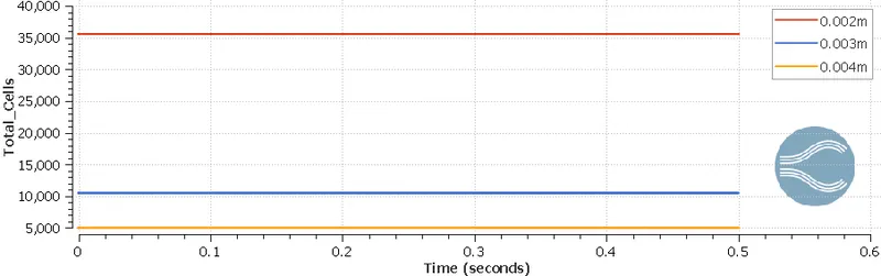
For the given case for a y+ of 10, the first cell size is 6.47e-4 and the estimated cell count is 12lakhs which is greater than the license provided hence we go with standard sizes like 0.004,0.003,0.002.
- In the Output/Post-processing section > Output files > writing time intervals tab > set the time interval for writing 3d output files to 0.01s this will make sure that the files are written for every 0.01s thereby we have more data and more clear curves.
- The time interval for writing the text output is 1e-6s This prints the text output on the command window.
- The time interval for writing the restarting output file. The restart file can be used to restart the simulation from a particular moment without having to start the simulation from the starting in case of any unexpected events like power loss, Out of memory etc. But writing it every time step takes time and energy so for our convenience, we write it every 0.04s. Press ok.
Save the case setup, upon pressing ctrl+S we save the case setup file which has a .cvg extension.
EXPORTING THE FILES
Now since the case is set, we need to run the simulation. Save this case file on the local computer and then go to the “taskbar on the top left” > file > export > export input files. We should see total of 12files. The usual location is set to the same directory where the case file is saved. Set the location and export the files.
RUNNING THE SIMULATION
Open the Cygwin terminal as administrator and navigate to the location where the case files are stored using the cd command. Then we execute the following command.
mpiexec.exe -n 4 converge.exe restricted </dev/null> logfile.txt &
mpiexec.exe is the message passing interface executive file.
-n 4 represents the number of cores to be used for running the simulation.
converge.exe is the converge file that runs the simulation.
restricted limits the total number of cells to 5,00,000
Now we can see many lines being printed on the Cygwin terminal. We can stop this process by pressing Ctrl + C in the Cygwin terminal. We go to the “inputs” file in the case directory, In the outputs control > log level > 0. Now run the above command again in the terminal. This should reduce the amount of output being printed in the Cygwin terminal.
This is done to know the control of the level of output being printed on the Cygwin terminal. Once the simulation is finished, we need to post-process the files.
POST-PROCESSING
We open converge > on the bottom left there are some options like postprocessing, lines etc. We select the post-processing and that will take us to a new window. Here we select the location of the output file which is created in the same directory in which we stored the input files. Once the output file is selected a list appears in the window below the file location option > click on select all and the below the cell variables will be listed > click on select all. Above the file location option, there is space for naming the post-processed file we give a proper name (preferably without spaces/special characters). And then select the output format as “Para-view vtk inline binary”. Once we do this the click convert. And the files will be post-processed.
Once the post-processing is done open Para-view > open file select the output file location > select the converted file _..vtm – group file. This will load the results in Para-view. Click on apply to view the case we setup.
In the top panel select the surface with edges to view the mesh and we might see that with the mesh there are some diagonal lines visible on the mesh. This is because the triangle converge created. So, we create a slice of this geometry. This slice will have the normal in x/y direction. For this in the top panel in the bottom-most line of the top panel, there is an option called slice we select that and then click on x/y-normal and apply. This will create a slice of the geometry. In the top toolbar, there is an option called surface with edges select it. This will show the mesh
The mesh on the slice would look like this
0.004m 0.003m 0.002m
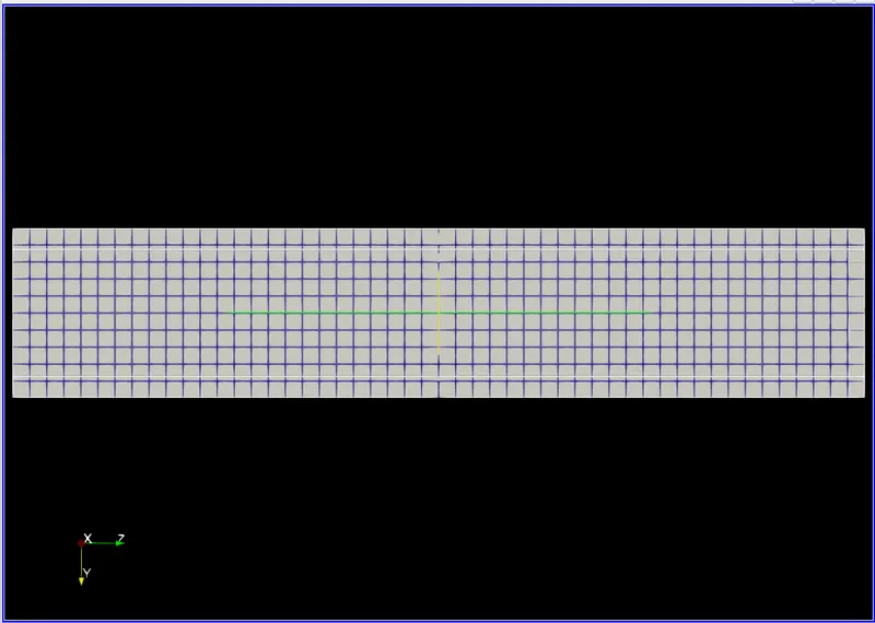
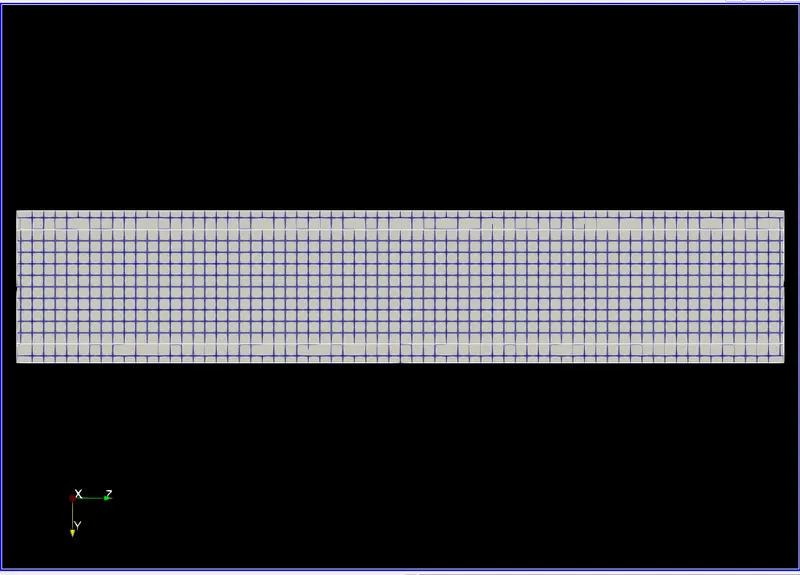
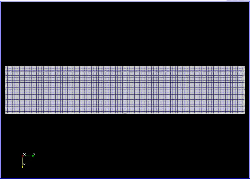
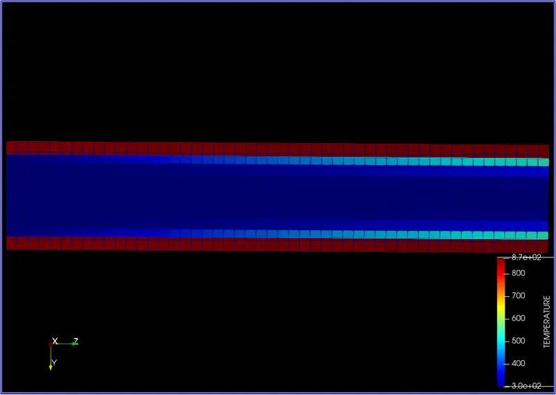
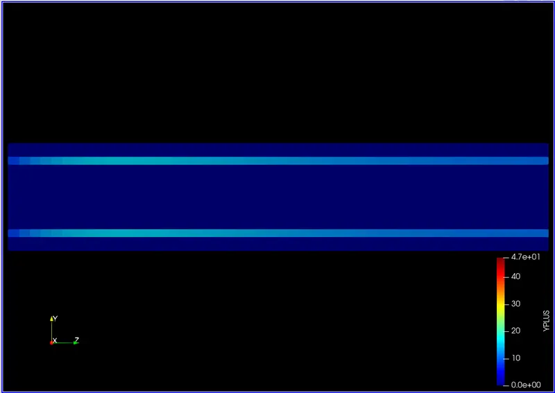
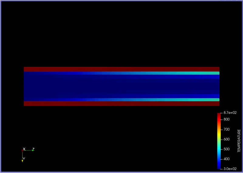
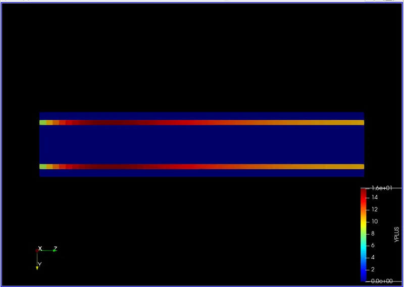
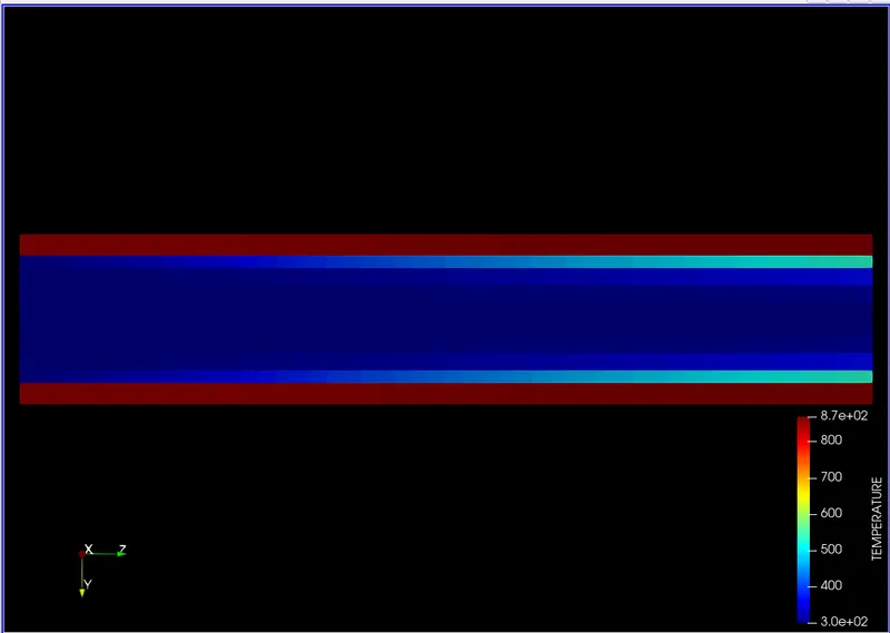
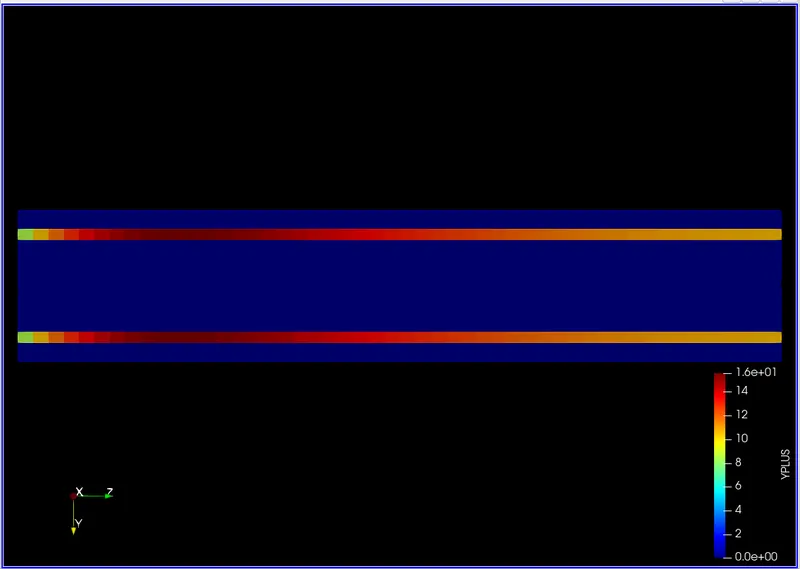
Now for the slice to the left of the surface option, there is another option which might be something like vtkblockcolors or idreg or solid color. Here, select a parameter, this will show the parameter’s contour at each time. Click the play button on the top. Upon selecting the Temperature, we can see the Temperature contour. If we select y+ we can how y+ varies along the length of the pipe
contour for different super cycling intervals. For super cycling a grid size of 0.004m is taken for all intervals
0.01
0.02
0.03
0.05
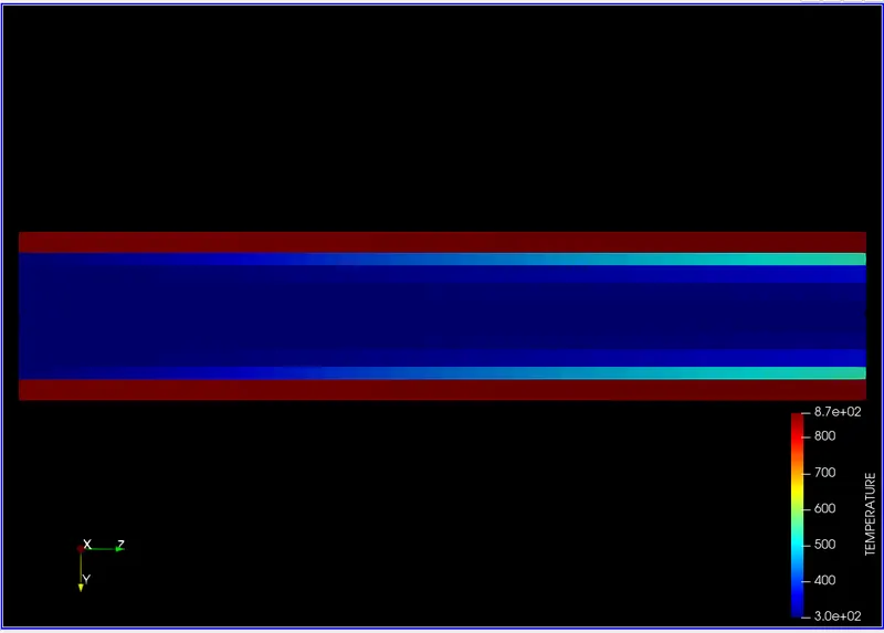
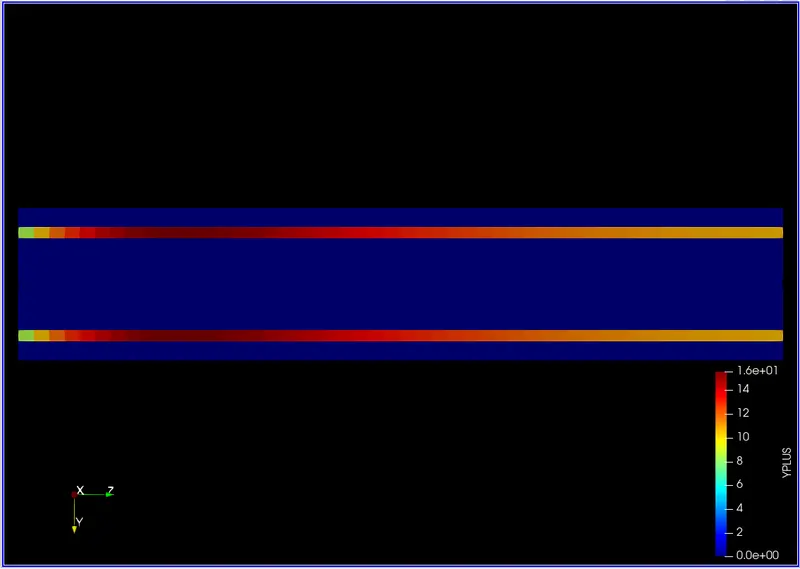
We can see that for the given grid size the y+ is not below 10 and it changes as velocity changes.
The animation of all the time steps can be saved using the save animation option
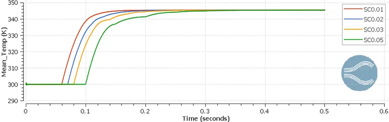
We can also use some of the converge features to compare results. In converge on the bottom left beside the post-processing, there is another tab called line plotting. Upon clicking this it will take us into another window. Here we select the same location where we saved the case setup file. This is because the converge takes the .out files as the input upon selecting the file location some variables are displayed in the window below. We select the file as massflowrate.out. The x axis will be cycles and on the y axis, we can select Temperature, Velocity etc.
These are the graphs we generated using the converge line plotting module.
Mean temperature Fluid region for different super cycling integrals
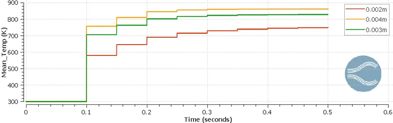
Mean temperature Solid region for different super cycling integrals
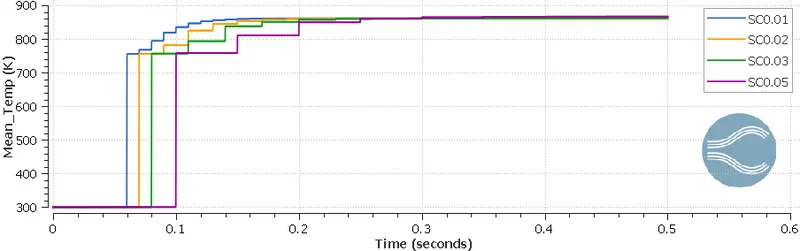
For different super cycling intervals, the total simulation time are as follows
| Super cycling time interval | Total time taken for simulation |
| 0.01 | 133.914877s |
| 0.02 | 132.562555s |
| 0.03 | 136.513493s |
| 0.05 | 141.857662s |
Mean temperature Fluid region for different grid sizes(the orange graph represents the 0.004m grid size)
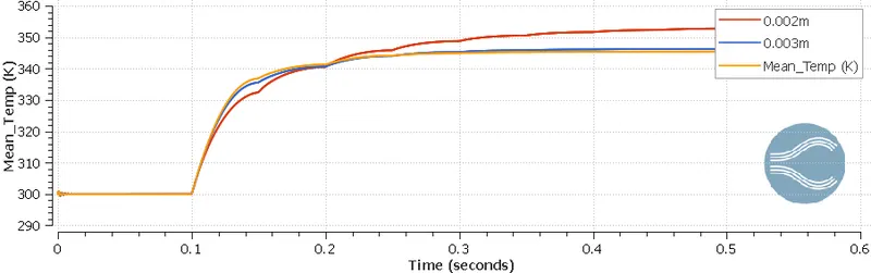
Mean temperature Solid region for different grid sizes
Total cell count for different grid sizes
CONCLUSION
The following conclusions have been made after observing the above plots and results
- The super cycling interval doesn't seem to affect the end solution.
- As the super cycling interval increases the total simulation time increases.
- The solution seems to be grid-dependent.
- The y+ value is not constant along the length this is because the y+ is dependent on the velocity which changes along the length.
REFERENCES