Week 6: Conjugate Heat Transfer Simulation

Aim:

To setup a transient state Conjugate Heat Transfer simulation of flow through a pipe in converge by using different stage interval for super cycling model and different grid size, simulate it using Cygwin terminal and post process in Paraview and check the results.

Conditions:

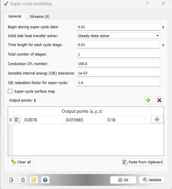
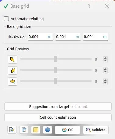
base :- dx=0.004, dy=0.004, dz=0.004 : supercyle stage interval = 0.04

case 1:- dx=0.003, dy=0.003, dz=0.003 : supercyle stage interval = 0.03

case 2:- dx=0.002, dy=0.002, dz=0.002 : supercyle stage interval = 0.02

case 3:- dx=0.001, dy=0.001, dz=0.001 : supercyle stage interval = 0.01

Conjugate Heat Transfer:

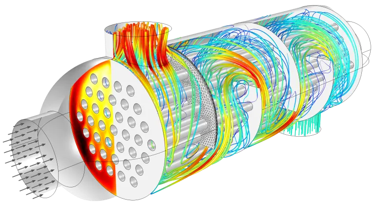
Conjugate heat transfer is a type of heat transfer analysis between solids and fluid(s). This type of heat transfer includes both convection (between fluids) and conductive (between solids) heat transfer, as well as both forced and natural convection.

Heat Transfer in a Solid:

• In most cases, heat transfer in solids, if only due to conduction, is described by Fourier’s law defining the conductive heat flux, q, proportional to the temperature gradient: `q=-k∇T`
• For a time-dependent problem, the temperature field in an immobile solid verifies the following form of the heat equation:

`ρC_p ( ∂T)/(∂t)=∇.(k∇T)+Q`

Heat Transfer in a Fluid

Due to the fluid motion, three contributions to the heat equation are included:

1. The transport of fluid implies energy transport too, which appears in the heat equation as the convective contribution. Depending on the thermal properties on the fluid and on the flow regime, either the convective or the conductive heat transfer can dominate.
2. The viscous effects of the fluid flow produce fluid heating. This term is often neglected, nevertheless, its contribution is noticeable for fast flow in viscous fluids.
3. As soon as a fluid density is temperature-dependent, a pressure work term contributes to the heat equation. This accounts for the well-known effect that, for example, compressing air produces heat.

Accounting for these contributions, in addition to conduction, results in the following transient heat equation for the temperature field in a fluid:

`nbsp; `ρC_p (∂T)/(∂t)+ρC_p u.∇T=α_p T((∂pA)/(∂t)+u.∇pA)+τ:S+∇.(k∇T)+Q`

Efficiently combining heat transfer in fluids and solids is the key to designing effective coolers, heaters, or heat exchangers.

Calculation:

Reynold's number Re = 7000

Density of air, ρ = 1.177 kg/m3 [for 300k]

Diameter of the pipe, d=0.03

Dynamic viscoity, `μ` =1.86e-5[fro 300k]

`Re = (ρvd)/μ`

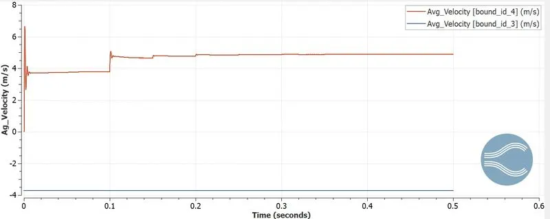
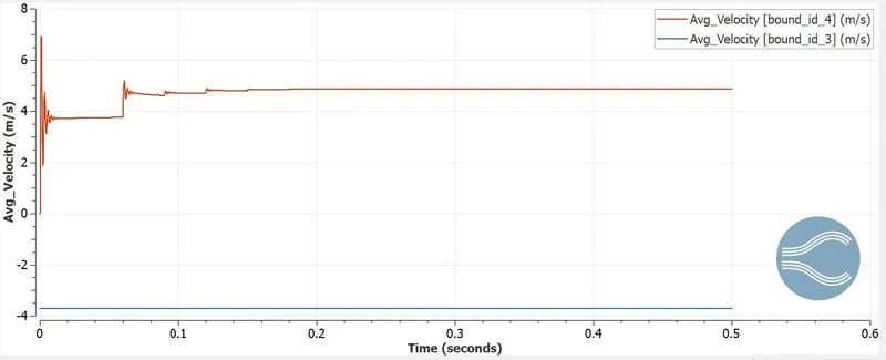
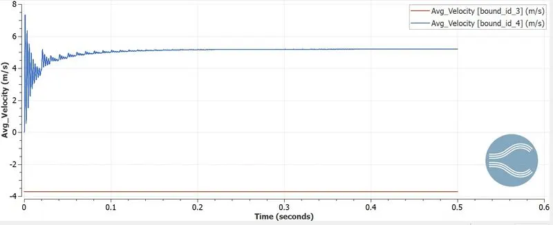
Hence, Inlet Velocity, v=3.71 m/s

Total simulation time:

Length of the pipe = 0.2m

Inlet velocity, v = 3.71 m/s

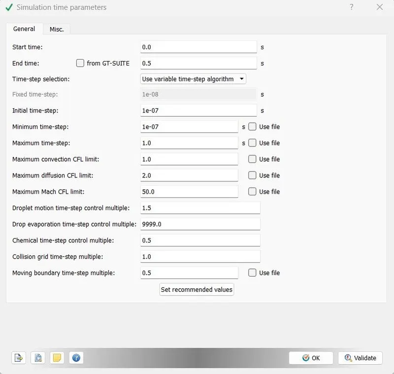
Total time required for single flow cycle = L/v = 0.2/3.71 = 0.05 s

Total time equired for 10 flow cycle = 0.05*10 = 0.5

hence, End time taken, t= 0.5 s

Procedure:

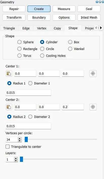
• Open Converge and generate the required pipe geometry using create->Shape select cylinder and put appropriate dimension and create the geometry.

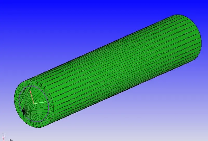
• Assign the appropriate boundary flag "Solid outer wall, Solid side, Inlet, Outlet, interface" and then check the normals.

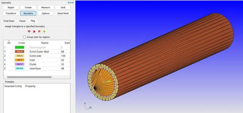
• After that setting the case set up one by one as per the requirements.

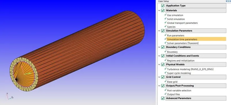
Materials:

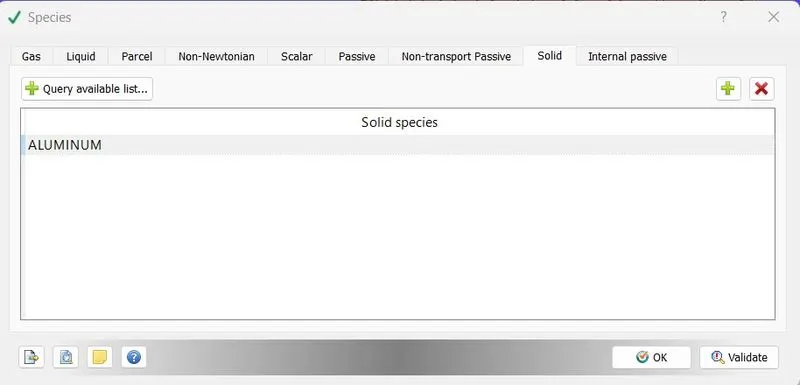
Solid - Aluminium

Fluid - Air

case setup:

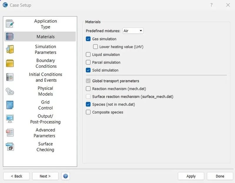
Solid Simulation:

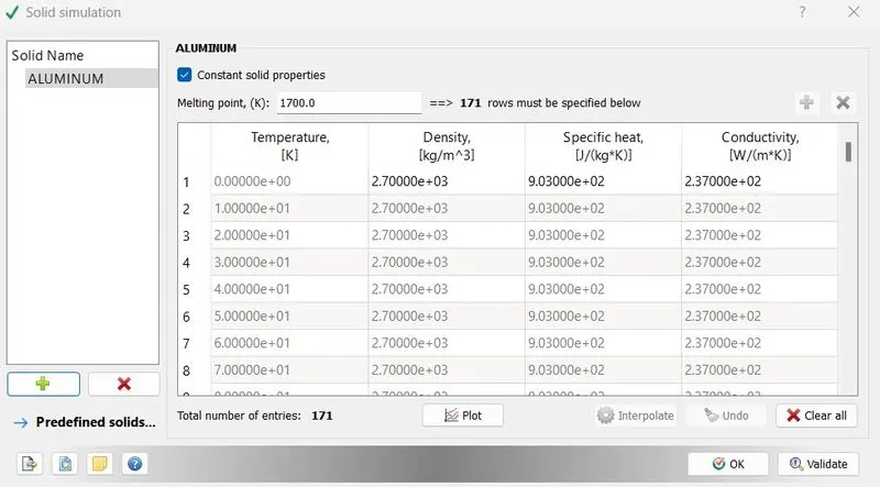
Species:

Fluid:

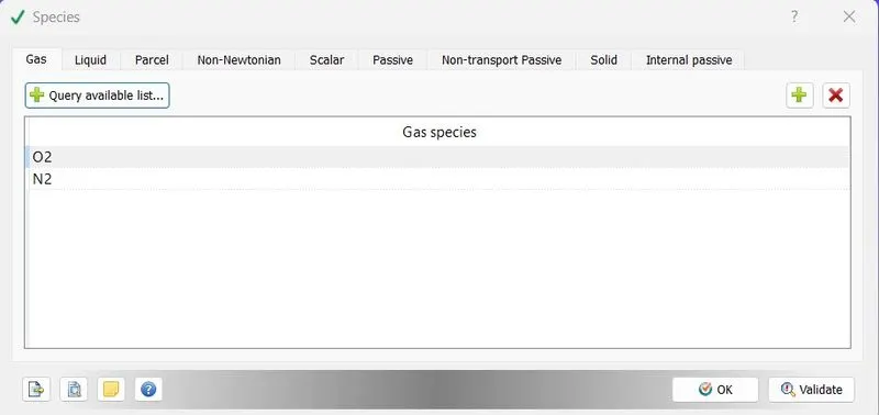
Solid:

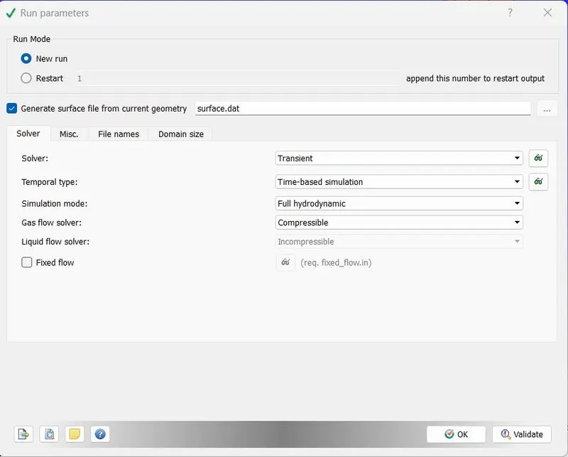
Run Parameter:

Simulation Time Parameter:

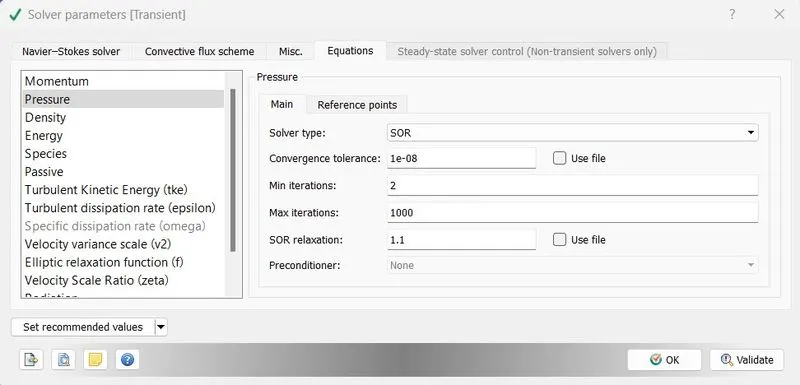
Solver Parameters:

Boundary conditions:

Solid Outer Wall:

Solid Side:

Inlet:

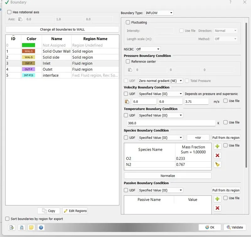
Outlet:

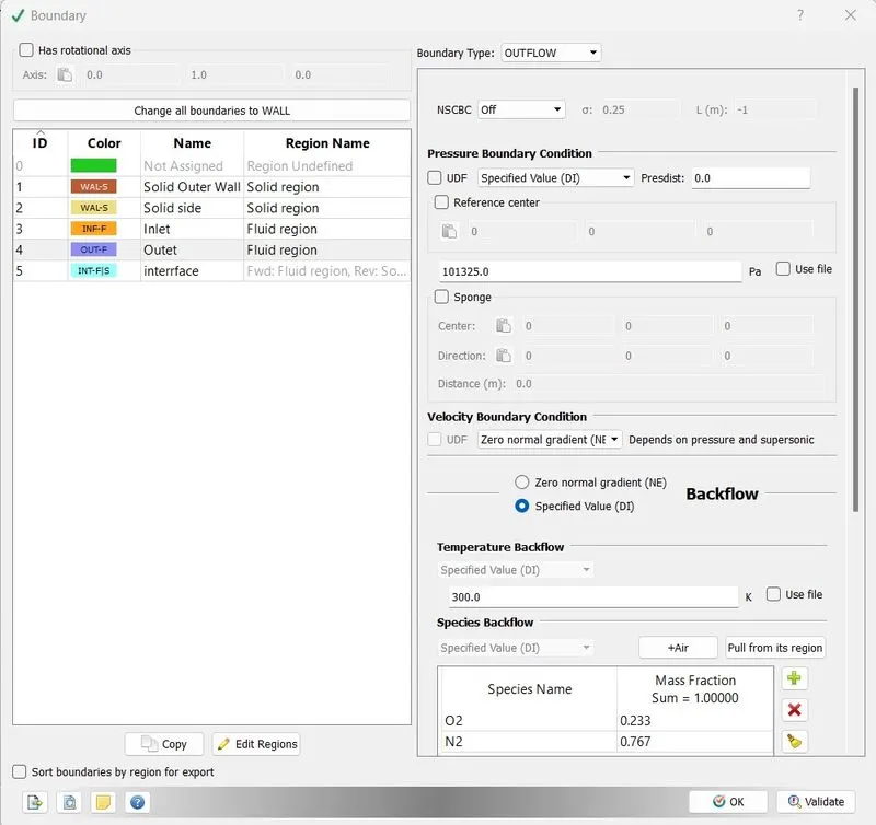
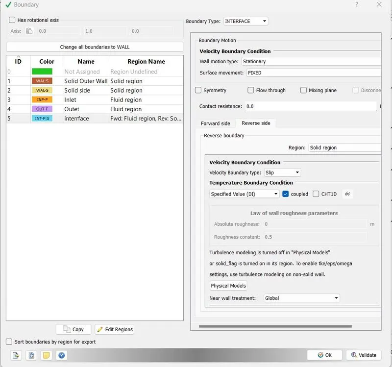
Interface:(Forward)

Interface:(Reverse)

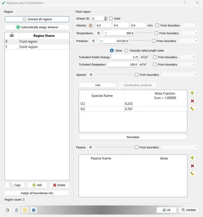
Regions:

Fluid Region:

Solid Region:

Physical Models:

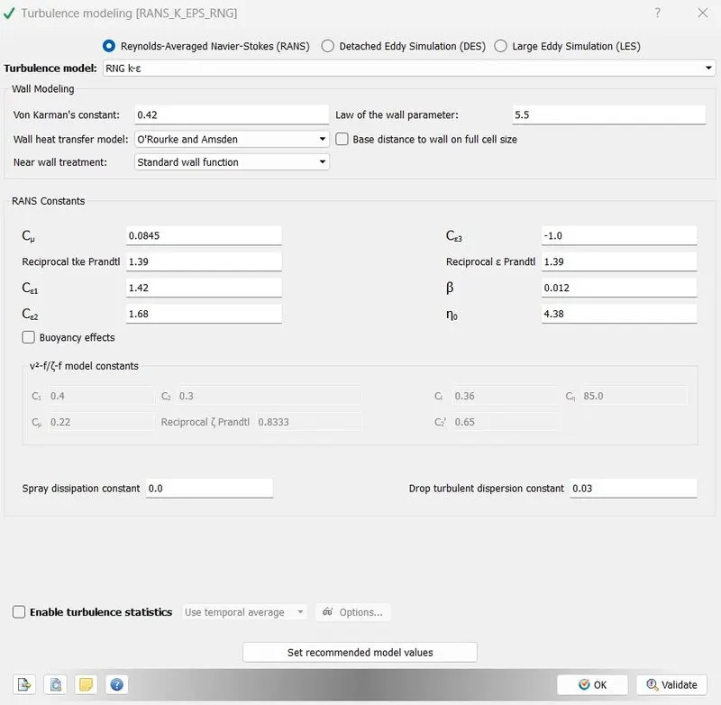
Turbulence Modeling:

Super-cycle Modeling:

Grid Control:

• Repeat the same procedure with different grid size and super cycle stage interval value.

base :- dx=0.004, dy=0.004, dz=0.004 : supercyle stage interval = 0.04

case 1:- dx=0.003, dy=0.003, dz=0.003 : supercyle stage interval = 0.03

case 2:- dx=0.002, dy=0.002, dz=0.002 : supercyle stage interval = 0.02

case 3:- dx=0.001, dy=0.001, dz=0.001 : supercyle stage interval = 0.01

Output files:

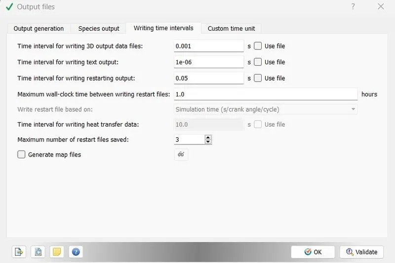
• After setting up the case setup export all the input files in specific location.

Export:

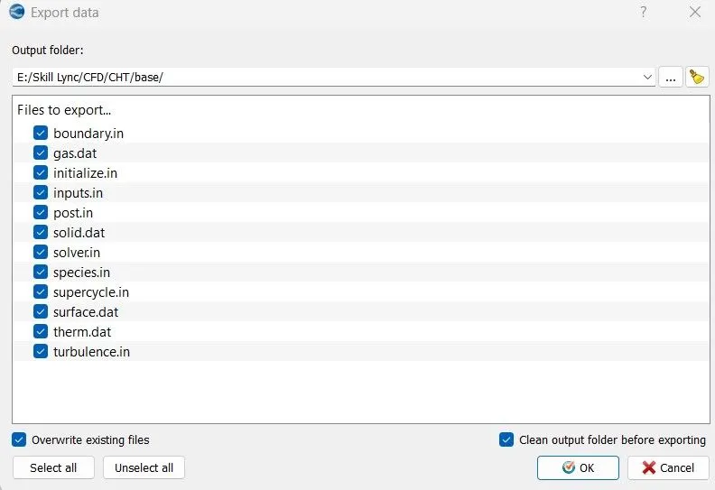
• Then open Cyqwin, navigate to the input files were located then run the simulation for different grid size and super cycle stage interval, observe and compare the results.
• It will take sometime to complete the simulation. After successfully completed the simulation post convert the results so that we can observe the results in paraview.

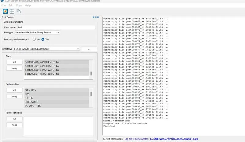
• Make some required plots in converge and some profile in paraview and create an animation in paraview.

Results:

base :- dx=0.004, dy=0.004, dz=0.004 : supercyle stage interval = 0.04

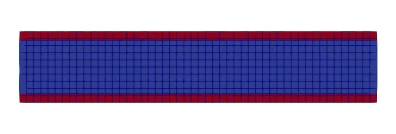
Mesh:

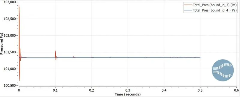
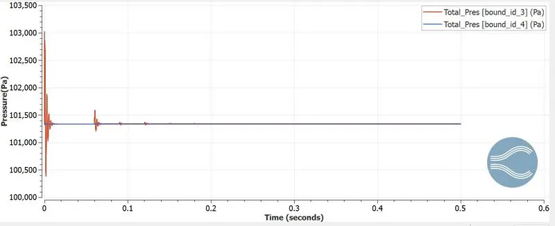
Pressure Plot:

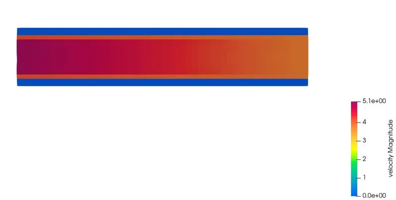
Velocity Plot:

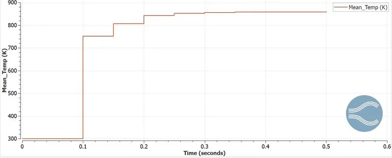
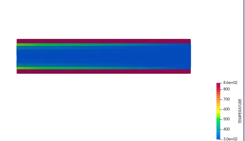
Temperature Plot:(solid)

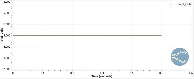
Total Cell Count:

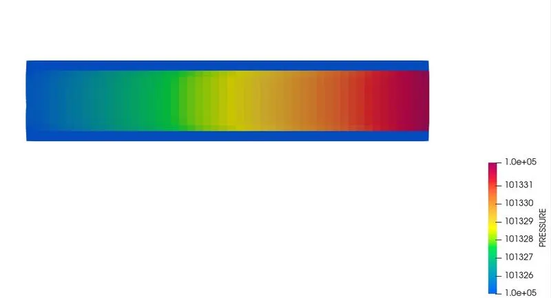
Pressure:

Velocity:

Temperature:

Animations:

Pressure:

Velocity:

Temperature:

case 1:- dx=0.003, dy=0.003, dz=0.003 : supercyle stage interval = 0.03

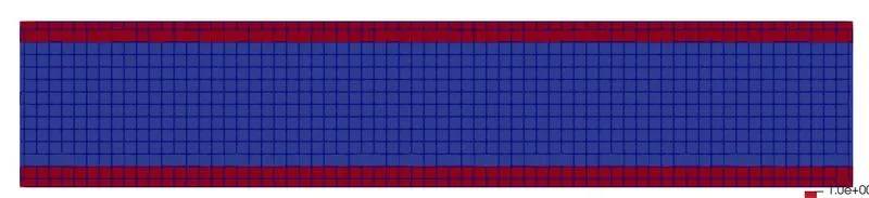
Mesh:

Pressure Plot:

Velocity Plot:

Temperature Plot:(solid)

Total Cell Count:

Pressure:

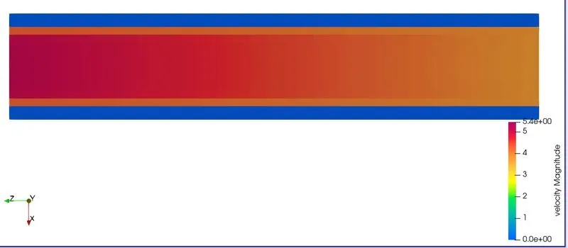
Velocity:

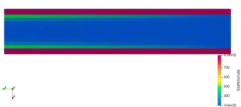
Temperature:

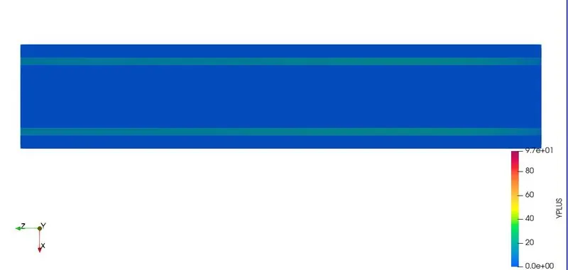
Y plus:

Animations:

Pressure:

Velocity:

Temperature:

case 2:- dx=0.002, dy=0.002, dz=0.002 : supercyle stage interval = 0.02

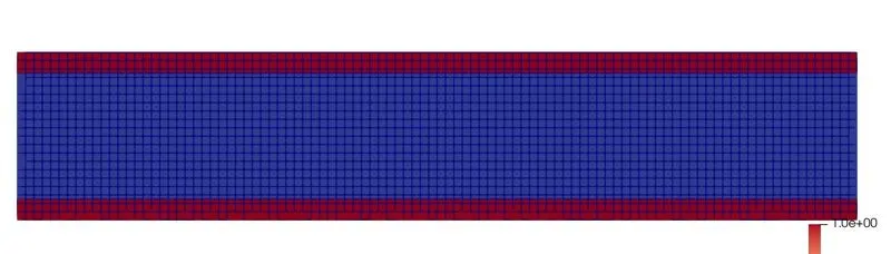
Mesh:

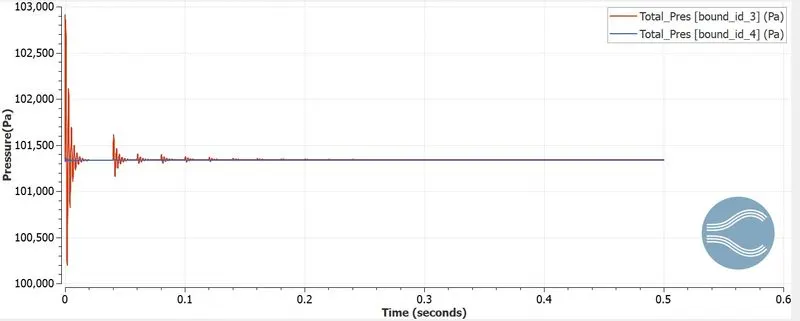
Pressure Plot:

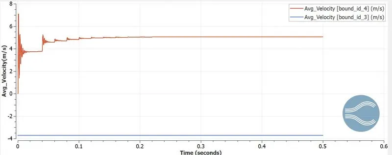
Velocity Plot:

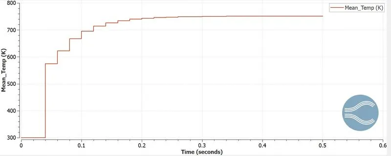
Temperature Plot:(solid)

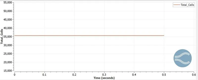
Total Cell Count:

Pressure:

Velocity:

Temperature:

Y plus:

Animations:

Pressure:

Velocity:

Temperature:

case 3:- dx=0.001, dy=0.001, dz=0.001 : supercyle stage interval = 0.01

Mesh:

Pressure Plot:

Velocity Plot:

Temperature Plot:(solid)

Total Cell Count:

Pressure:

Velocity:

Temperature:

Animations:

Pressure:

Velocity:

Temperature:

Conclusions:

• Transient conjugate heats transfer simulation of flow through a pipe is carried out for 0.5 seconds.
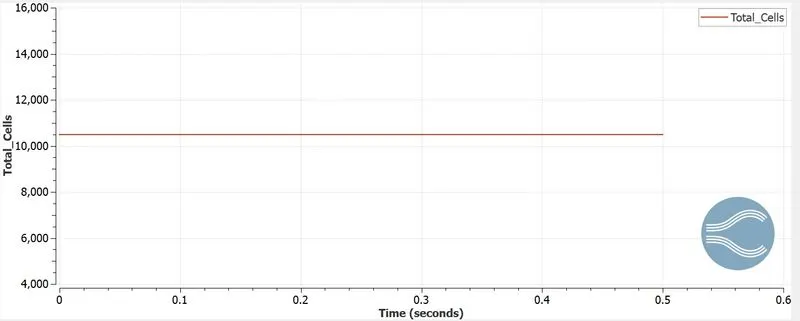
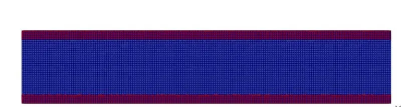
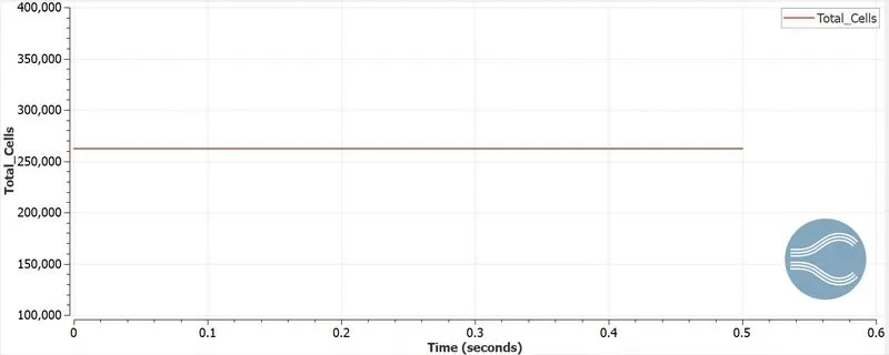
• Cut cell meshing strategy is used in converge studio. The total cell count for baseline, case 1, case 2 and case 3 are 5000, 10500, 36000 and 260000 respectively.
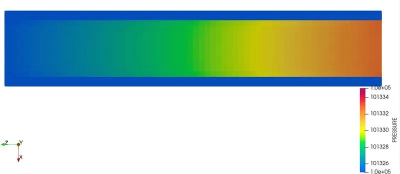
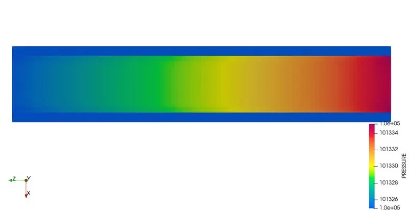
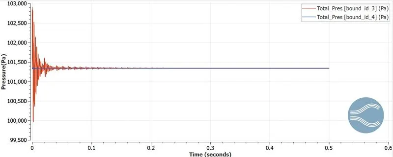
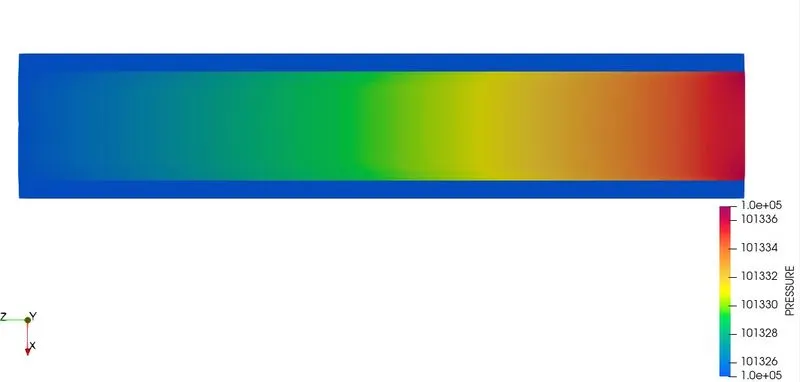
• Contour shows that the pressure is high at the inlet and gradually reduces at the outlet to the specified in the outlet boundary conditions.
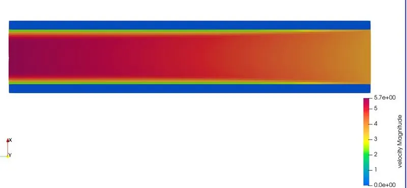
• Whenever the mesh size decreased the results get more accurate. Finer mesh can give accurate results and also take more time to run the simulation.
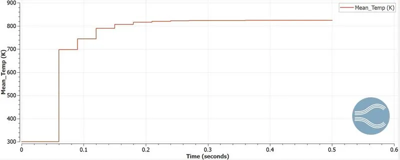
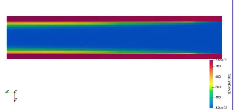
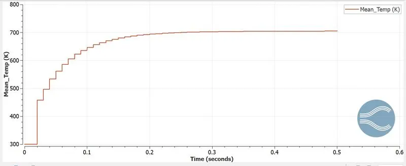
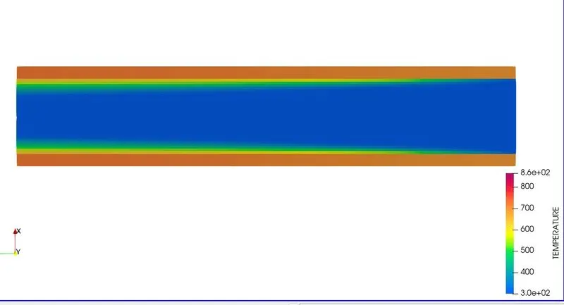
• Temperature contour and plot shows that the solid domain with different grid size of 0.004, 0.003 m, 0.002 m and 0.001 m attains different average temperature of 850 K, 820 K, 750 K and 700 k respectively.
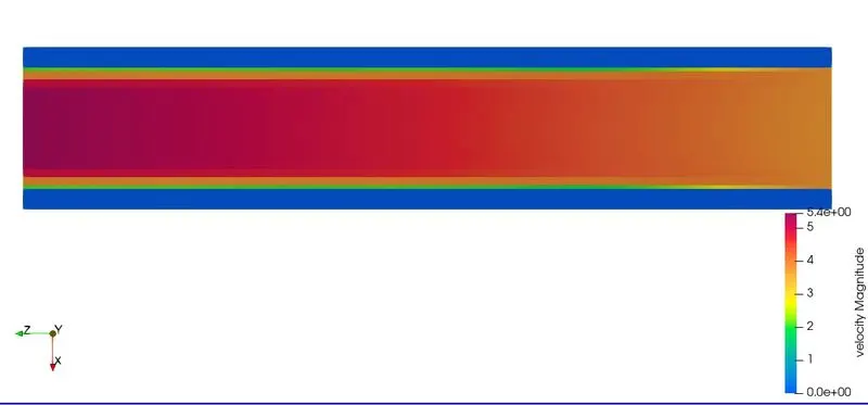
• The simulation correctly captures the physics of conjugate heat transfer clearly as it shows the heat flux applied on the solid outer wall transfers through the solid domain via conduction and then to the fluid domain via convection.