Week 4.1 - Genetic Algorithm

A code to optimise the stalagmite function and find the global maxima of the function.

Main program:

clear all
close all
clc

x = linspace(0,0.6,150);
y = linspace(0,0.6,150);
num_cases = 50;
[xx,yy] = meshgrid(x,y)

for i = 1:length(x);
    for j = 1:length(y);
        input_vector(1) = xx(i,j);
        input_vector(2) = yy(i,j);
        f(i,j) = stalagmite(input_vector);
    end
end

tic
for i = num_cases;
    [results,fopt(i)] = ga(@stalagmite,2);
    xopt(i) = results(1);
    yopt(i) = results(2);
end
study_time1 = toc
figure(1)
subplot(2,1,1)
surf(x,y,-f)
xlabel(Xaxis)
ylabel(Yaxis)
shading interp
hold on
plot3(xopt,yopt,-fopt,'marker','o')
subplot(2,1,2)
plot(-fopt)
xlabel('iteration')
ylabel('function maximum')

tic
for i = num_cases
    [results,fopt(i)] = ga(@stalagmite,2,[],[],[],[],[0;0],[0.6;0.6])
    xopt(i) = results(1)
    yopt(i) = results(2)
end
study_time2 = toc
figure(2)
subplot(2,1,1)
surf(x,y,-f)
shading interp
hold on
plot3(xopt,yopt,-fopt,'marker','o')
subplot(2,1,2)
plot(-fopt)
xlabel('iteration')
ylabel('function maximum')

tic
options = optimoptions('ga')
options = optimoptions(options,'populationsize',250)
for i = num_cases
    [results,fopt(i)] = ga(@stalagmite,2,[],[],[],[],[0;0],[0.6;0.6],[],options)
    xopt(i) = results(1)
    yopt(i) = results(2)
end
study_time3 = toc
figure(3)
subplot(2,1,1)
surf(x,y,-f)
shading interp
hold on
plot3(xopt,yopt,-fopt,'marker','o')
subplot(2,1,2)
plot(-fopt)
xlabel('iteration')
ylabel('function maximum')

Stalagmite Function(sub function):

function A = stalagmite(input_vector)
x = input_vector(1)
y = input_vector(2)

f1 = (sin(5.1*pi*x+0.5)).^6
f2 = exp((-4*log(2)-((x-0.0667).^2))/0.64)
f3 = (sin(5.1*pi*y+0.5)).^6
f4 = exp((-4*log(2))*((y-0.0667).^2)/0.64)

A = -(f1*f2*f3*f4)
end

• Starting few commands like ‘clear all’, ‘close all’, ‘clc’ are entered to clear any existing data from previous program or command section.
• Then enter the input values through commands such as x ,y and num_cases. Then create a 2d array using mesgrid command.
• Then enter the for loop command to get appropriate results and tic &tac command to get the time duration.
• Repeat the same process again and again running multiple iteration and Num_cases to get appropriate results.
• Then save and run the program to get results and plots.

Results And Plots:

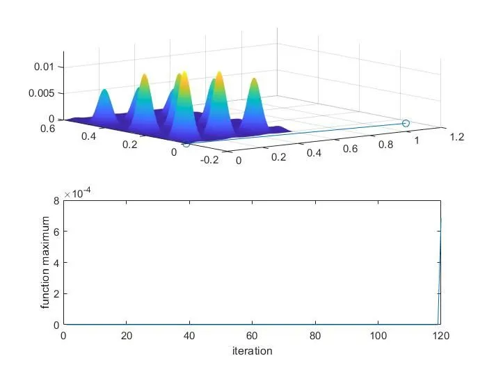
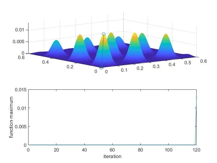
Genetic Algorithm(GA):

• A genetic algorithm (GA) is a method for solving both constrained and unconstrained optimization problems based on a natural selection process that mimics biological evolution. The algorithm repeatedly modifies a population of individual solutions. At each step, the genetic algorithm randomly selects individuals from the current population and uses them as parents to produce the children for the next generation. Over successive generations, the population "evolves" toward an optimal solution.
• You can apply the genetic algorithm to solve problems that are not well suited for standard optimization algorithms, including problems in which the objective function is discontinuous, nondifferentiable, stochastic, or highly nonlinear.

Stopping Criteria

• Proof of convergence of an algorithm to an optimal solution is very important as it assures the optimal solution in infinite iterations. When an algorithm does not assure or guarantee the optimal solution even after running for infinite iterations, it’s utility is in doubt. Once the convergence of an algorithm is assured, the focus turns into the exploration of stopping time or stopping criterion of the algorithm.

Synax:

[x,fval] = ga(@plotfunc,numberofvariales)

[x,fval] = ga(@plotfunc,numberofvariales,[],[],[],[],[],[])

opts = optimoptions(@ga,'PlotFcn',{@gaplotbestf,@gaplotstopping})

[x,fval] = ga(@plotfunc,numberofvariales,[],[],[],[],[],[],[],options)

significance of running multiple iterations;

• when we urunning a multiple ietrations we can get appropriate resuts without any error.