Project 2 - Rankine cycle Simulator

Aim:

To create a Rankine Cycle Simulator fro given input data from XSteam library.

Objective:

• To create a Rankine Cycle Simulator in MATLAB.
• To calculate the state point using function XSteam.
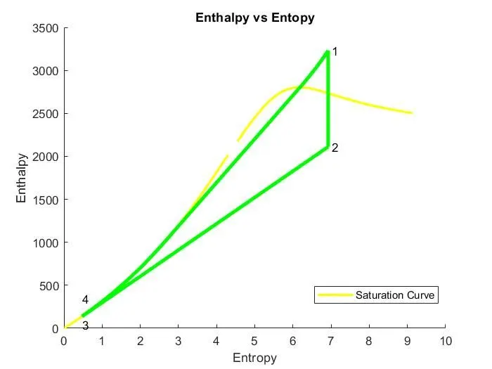
• To plot T-S and H-S diagram for given input in Rankine Cycle.
• To get output in the command window for each state point in cycle.

Description:

• The Rankine cycle closely describes the process by which steam engines commonly found in thermal power generation plants harness the thermal energy of a fuel or other heat source to generate electricity. Possible heat sources include combustion of fossil fuels such as coal, natural gas, or oil, renewable fuels like biomass or ethanol, nuclear fission, and concentrated solar power. Common heat sinks include ambient air above or around a facility and bodies of water such as rivers, ponds, and oceans.
• The ability of a Rankine engine to harness energy depends on the relative temperature difference between the heat source and heat sink. The greater the differential, the more mechanical power can be efficiently extracted out of heat energy, as per Carnot's theorem.
• The efficiency of the Rankine cycle is limited by the high heat of vaporization of the working fluid. Unless the pressure and temperature reach super critical levels in the boiler, the temperature range that the cycle can operate over is quite small: Steam turbine entry temperatures are typically around 565 °C and condenser temperatures are around 30 °C. This gives a theoretical maximum Carnot efficiency for the turbine alone of about 63.8% compared with an actual overall thermal efficiency of less than 50% for typical power stations. This low steam turbine entry temperature (compared to a gas turbine) is why the Rankine (steam) cycle is often used as a bottoming cycle to recover otherwise rejected heat in combined-cycle gas turbine power stations.

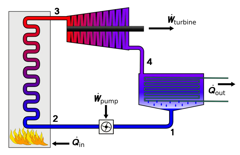
• Rankine engines generally operate in a closed loop where the working fluid is reused. The water vapor with condensed droplets often seen billowing from power stations is created by the cooling systems (not directly from the closed-loop Rankine power cycle). This 'exhaust' heat is represented by the "Q_out" flowing out of the lower side of the cycle shown in the T–S diagram below. Cooking towers operate as large heat exchangers by absorbing the latent heat of vaporization of the working fluid and simultaneously evaporating cooling water to the atmosphere.
• The process in Rankine Cycle are given as;

1. Isentropic Compression in Pump.
2. Constant pressure heat addition in Boiler.
3. Isentropic expansion in a Turbine.
4. Constant pressure heat rejection in Condenser.

Main program to create a Rankine Cycle:

clear all
close all
clc


fprintf("               RANKINE CYCLE    ")
fprintf("\n\n1-2 is Isentropic Expansion in the Turbine")
fprintf("\n2-3 is constant Pressure Heat Rejection by the condenser")
fprintf("\n3-4 is Isentropic Compression in the Pump")
fprintf("\n4-1 is constant Pressure Heat Addition by the Boiler\n")
fprintf('  \n')
%input data for state point 1
p1 = 30;
t1 = 400;
p2 = 0.05;
h1 = XSteam('h_pT',p1,t1);
s1 = XSteam('s_pT',p1,t1);
%input data for state point 2
s2 = s1;
sf2 = XSteam('sL_p',p2);
sg2 = XSteam('sV_p',p2);
hf2 = XSteam('hL_p',p2);
hg2 = XSteam('hV_p',p2);
x2 = ((s2-sf2)/(sg2-sf2));
h2 = hf2+(x2*(hg2-hf2));
%input data for state point 3
p3 = p2;
h3 = XSteam('hL_p',p3);
s3 = XSteam('sL_p',p3);
%input data for state point 4
p4 = p1;
s4 = s3;
%workdone in Turbine
W_T = h1-h2;
%workdone for Pump
v3 = XSteam('vL_p',p3);
W_P = v3*(p4-p3)*100;
h4 = h3+W_P;
%net workdone
W_net = W_T-W_P;
%Heat addition
Q_in = h1-h4;
%Heat rejection
Q_out = h2-h3;
%Thermal efficiency
T_eff = (W_net/Q_in)*100;
%Specific steam consumption = (Mass flow rate / Net workdone)
Sp_S = (3600/W_net);
%Calculation of temperature at all state points
t3 = XSteam('Tsat_p',p3);
t2 = t3;
cp4 = XSteam('Cp_ps',p4,s4);
cv4 = XSteam('Cv_ps',p4,s4);
g = cp4/cv4;
o = (g-1)/g;
t4 = t3*((p4/p3)^o);
%constants for saturated liquid and vapour
t6 = XSteam('Tsat_p',p1);
s5 = XSteam('sL_p',p1);
s6 = XSteam('sV_p',p1);
h5 = XSteam('hL_p',p1);
h6 = XSteam('hV_p',p1);
t5 = t6;

%plotting saturated line
T = linspace(1,500,1000);
for i = 1:length(T)
    sf(i) = XSteam('sL_T',T(i));
    sg(i) = XSteam('sV_T',T(i));
    hf(i) = XSteam('hL_T',T(i));
    hg(i) = XSteam('hV_T',T(i));
end
% plotting T-S diagram
figure (1)
hold on
plot(sf,T,'Color','y','LineWidth',2)
plot(sg,T,'Color','y','LineWidth',2)
plot([s1 s2],[t1 t2],'Color','g','LineWidth',3)
plot([s2 s3],[t2 t3],'Color','g','LineWidth',3)
plot([s3 s4],[t3 t4],'Color','g','LineWidth',3)
plot([s4 s5],[t4 t5],'Color','g','LineWidth',3)
plot([s5 s6],[t5 t6],'Color','g','LineWidth',3)
s_1 = linspace(s6,s1,500);
for j = 1:length(s_1)
    Tc(j) = XSteam('T_ps',p1,s_1(j));
end
plot(s_1,Tc,'Color','g','LineWidth',3)
text(s1+0.1,t1,'1')
text(s2+0.1,t2,'2')
text(s3,t3-20,'3')
text(s4,t4+20,'4')
title('Temperature vs Entropy')
xlabel('Entropy (Kj/kg-k)')
ylabel('Temperature (Deg. Celcius)')
legend('saturated curve')
%plotting H-S diagram
figure(2)
hold on
plot(sf,hf,'Color','y','LineWidth',2)
plot(sg,hg,'Color','y','LineWidth',2)
plot([s1 s2],[h1 h2],'Color','g','LineWidth',3)
plot([s2 s3],[h2 h3],'Color','g','LineWidth',3)
plot([s3 s4],[h3 h4],'Color','g','LineWidth',3)
hc = linspace(h4,h5,100);
for k = 1:length(hc)
    s_c(k) = XSteam('s_ph',p1,hc(k));
end
plot(s_c,hc,'Color','g','LineWidth',3)
plot([s5 s6],[h5 h6],'Color','g','LineWidth',3)
for l = 1:length(s_1)
    h_c(l) = XSteam('h_ps',p1,s_1(l));
end
plot(s_1,h_c,'Color','g','LineWidth',3)
text(s1+0.1,h1,'1')
text(s2+0.1,h2,'2')
text(s3,h3-100,'3')
text(s4,h4+200,'4')
title('Enthalpy vs Entopy')
xlabel('Entropy')
ylabel('Enthalpy')
legend('Saturation Curve')

%display results
disp('Results of Rankine Cycle')
fprintf('  \n')
fprintf('At state point 1\n')
fprintf('  \n')
fprintf('P1 = %f in Bar\n',p1);
fprintf('T1 = %f in Deg.Celcius\n',t1);
fprintf('H1 = %f in KJ/kg\n',h1);
fprintf('S1 = %f in KJ/kg-k\n',s1);
fprintf('  \n')
fprintf('At state point 2\n')
fprintf('  \n')
fprintf('P2 = %f in Bar\n',p2);
fprintf('T2 = %f in Deg.Celcius\n',t2);
fprintf('H2 = %f in KJ/kg\n',h2);
fprintf('s2 = %f in KJ/kg-k\n',s2);
fprintf('  \n')
fprintf('At state point 3\n')
fprintf('  \n')
fprintf('P3 = %f in Bar\n',p3);
fprintf('T3 = %f in Deg.Celcius\n',t3);
fprintf('H3 = %f in KJ/kg\n',h3);
fprintf('S3 = %f in KJ/kg-k\n',s3);
fprintf('  \n')
fprintf('At state point 4\n')
fprintf('  \n')
fprintf('P4 = %f in Bar\n',p4);
fprintf('T4 = %f in Deg.Celcius\n',t4);
fprintf('H4 = %f in KJ/kg\n',h4);
fprintf('S4 = %f in KJ/kg-k\n',s4);
fprintf('  \n')
fprintf('Turbine Work Done   = %f in KJ/kg\n',W_T)
fprintf('Pump Work Done      = %f in KJ/kg\n',W_P)
fprintf('Net Work Done       = %f in KJ/kg\n',W_net)
fprintf('Thermal Efficiency  = %f in Percentage\n',T_eff)
fprintf('Sp.Steam Consumtion = %f in KJ/Kw',Sp_S)

Code Explanation:

• To create a Rankine Cycle Simulator starts with some basic commands such as ‘clear all’, ‘close all’, ‘clc’ to clear all data if there anything in previous program.
• Then enter some nput value which are required to calculate the other state point in cycle.
• The inputs which are input pressure and temperature for the turbine and inlet pressure at condenser.
• Then use the Xsteam function file for reading the state point.
• As process from 1-2 Isentropic compression so the entropy at point 1 is equal to point 2. The code ‘s_pT,p1,T1’ refers to entropy at pressure and temperature point 1.
• The term ‘sg’ and ‘sf’ are referred to saturated liquid and saturated vapor entropy respectively. This value is used to calculated other function according to mathematical relations.
• Repeat the same process further to get other points from XSteam function file which are necessary to calculate other parameters. Then the work done in turbine and pump are calculated to get net work done of Rankine Cycle.
• After calculating the net work done the efficiency of the Rankine Cycle is calculated along with specific steam consumption.
• Then all the temperature are calculated using the data from the XSteam funtion.
• Then create plots which is represent the T-S and H-S diagram and another loop program is used to create the saturation curve in each plot.
• Then enter the command ’fprintf’ to display all values in command window.

Results and Pots:

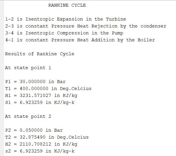
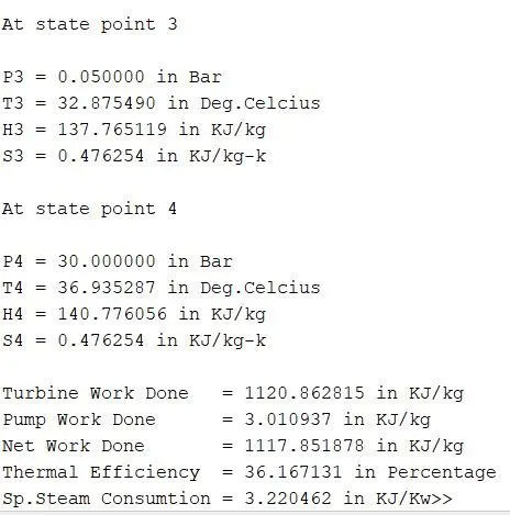
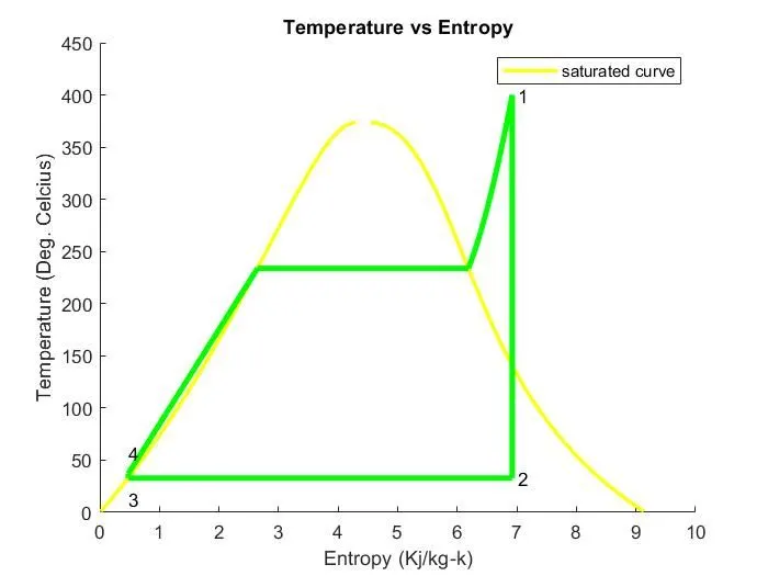
Conclusion:

Thus the Rankine Cycle Simulator were created and the state points were calculated with the help of XSteam data library file.