Week 6: Conjugate Heat Transfer Simulation

• Conjugate Heat Transfer Simulation
• Objective -To simulate the flow through the solid pipe "Conjugate Heat transfer" and understand super cycling.
• Introduction
  • Heat transfer coefficient
  • Give a brief description of why and where a CHT analysis is used.
  • It is a heat transfer analysis between solids and fluids.
  • This type of heat transfer includes both convective (liquid-to-liquid) and conductive (solid-to-solid) heat transfer, and both forced and natural convection.
  • The heat transfer simulation type allows you to calculate temperature distribution and heat flow in solids subjected to thermal stresses (such as convection and radiation).
  • A convective heat transfer analysis can be used when the temperature of a liquid changes its density.
  • Typical applications for this type of analysis include heat exchanger simulation and electronic device cooling,Purpose cooling and heating system.
  • Conductive heat transfer is heat transfer due to molecular excitation within a material without bulk mass transfer.

• Understanding wall functions and y+

• The wall function helps tell the solver how to approach the solution near the wall. They are used to accurately predict results near walls even on a coarse grid. There are several wall functions for each turbulence model, but the most basic is the standard wall function.
• The wall function approach saves significant computational resources because it does not need to solve the problem affecting viscosity in the near-wall region where the solution variables change fastest. The wall function approach is popular because it is economical, robust, and reasonably accurate. This is a practical option for near-wall processing for industrial flow simulations.
• However, the wall function approach is inadequate in situations where the effect of low Reynolds numbers in the flow regime is so widespread that the underlying hypothesis of the wall function loses its validity.
• In such situations, we need a near-wall model that is effective in the viscosity-affected region and integrates up to the wall accordingly. It is approximately the Reynolds number. Values ​​less than 1 are required to resolve laminar sublayers.
• The y+ value is directly related to the physical distance of the first cell from the wall. If you want a higher y+ move the first cell or grid point away from the wall, if you want a lower y+ decrease the distance by. It is a function of fluid properties and skin friction coefficient.

• Supercycling Concept
• Supercycling is the method used in Converge Studio for conjugate heat transfer problems in solid and liquid domains. The main problem is that both solvers cannot run at the same speed. This is because the solution is much faster in the liquid domain due to the difference in timescales of heat transfer in solids and liquids. This causes problems during the analysis because the solid side solver did not reach/converge when the liquid side solver reached steady state. The supercycling concept is based on this.
• The basic idea of ​​supercycling is to pause the fluid domain solver until the solid domain solver converges. The following steps are required to perform super cycling:
• Solve liquids and solids together with the transient solver. Store the instantaneous heat transfer coefficient and temperature in the interface during the process.
• Freeze Liquid Solvent. Temporarily average the heat transfer coefficient and temperature and apply it as a boundary condition.
• Solve until the solid temperature is steady state.
• Update fixed temperature field and release fluid solver.
• Repeat until the fixed temperature converges.

• Dittus Boelter equation
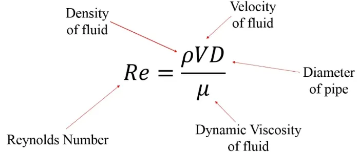
• This correlation is the so-called Dittus–Boelter correlation given as. Nu DB = 0.023 Re 0.8 Pr 0.4.
• Reynolds number

• Prandtl number

where, = Prandtl number

= momentum diffusivity

= thermal diffusivity

• Nusselt number

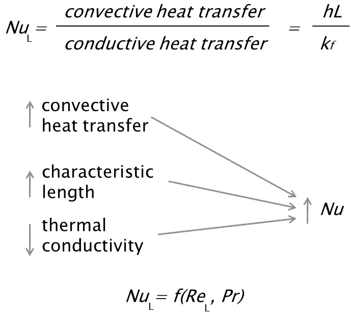
• Heat transfer coefficient

where , h = heat transfer coefficient

= Heat flux

= difference in temperature between a solid surface and surrounding fluid

• Procedure

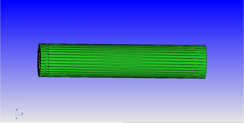
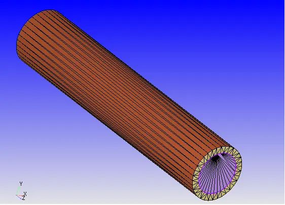
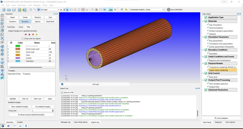
• Creating Geometry

• Setup

• Stepwise Explaination
• Geometry:
  
  Inner Diameter = 0.03 m
  
  Thickness Diameter = 0.01 m
  
  Tube Length = 0.2 m
• A diagnostic check is performed to check for errors in triangular elements touching each other, but this is normal simulation. Not recommended for However, it is unavoidable in CHT analysis. This error will automatically disappear after the case setup process as Converge identifies this simulation as a CHT analysis.
• To start case setup, click Case Setup, click Start Case Setup, and then click Time Based.
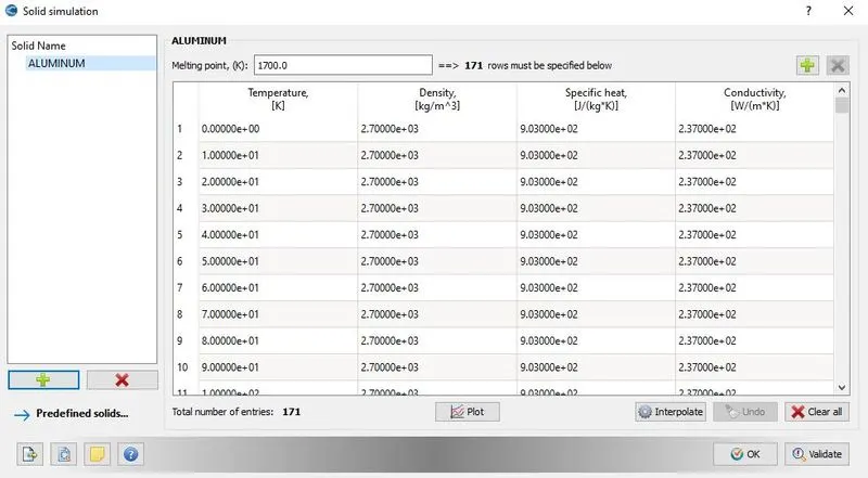
  Next, click Materials and select Air as the predefined mixture. Also activate solid simulation and seeds. Then open the gas simulation and global transport parameters and leave the default settings.
• Then open the Species tab and select Aluminum as the solid species from the Query Available list. Then go to Gas and select N2 and O2 as gas types from the Available Queries list.
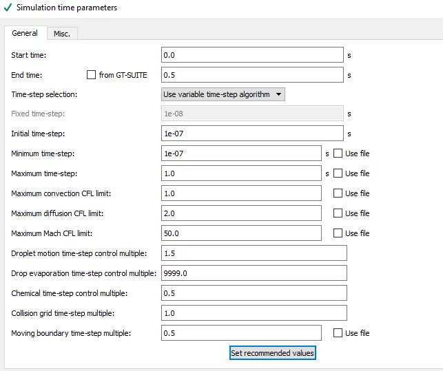
• Next, under Simulation Parameters, click Run Parameter, under the Solver tab select Transient Solver, under Simulation Mode select Full Hydrodynamic. Then select compressibility in the gas flow solver.
• For the solver time parameter, select only pressure-based solvers and keep the rest of the settings.
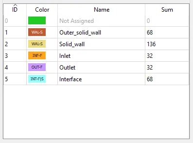
• Click Create Multiple Boundaries to add boundaries, create all boundaries at once, select the appropriate triangles, and and so on.
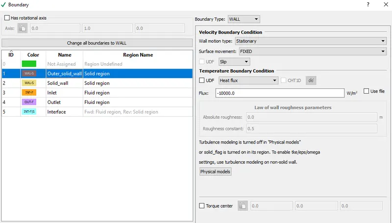
• Under Exterior, select Wall as the boundary type. And select -10000 as the heat flow for the temperature boundary condition. Also, select the area as solid area. For solid walls, select a wall type boundary condition. Select slip as the velocity boundary condition. Also a temperature boundary condition with zero normal slope. Also select the region as a solid region.
• Select boundary type as Inflow. Also select the region as the fluid region. Select a normal slope of zero for the pressure boundary condition. In Velocity Constraint, select 3.71 m/s in positive z. Then select 300K for the temperature boundary condition.
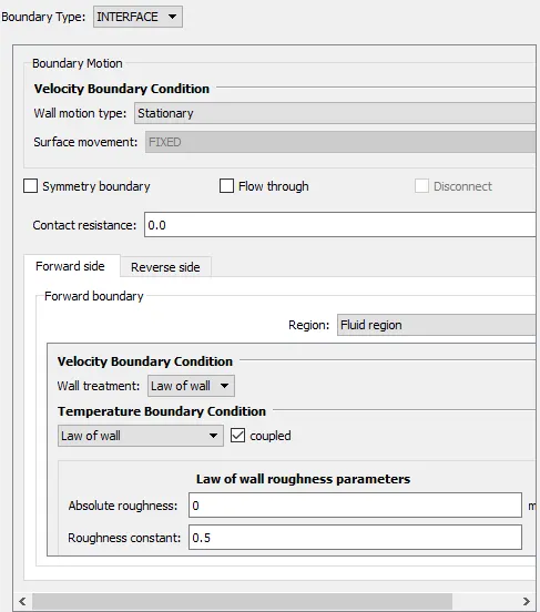
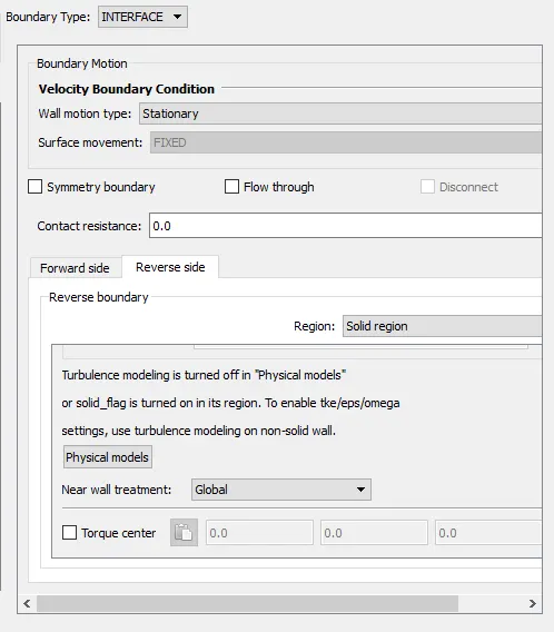
• Select Drain as Boundary Type and Region as Fluid Region. The pressure limit is given as 101325 Pa. And choose the velocity constraint as normal gradient zero. Choose a temperature of 300 K as the reflux boundary condition. And for seed return we choose air. An interface has a forward direction and a reverse direction.
• Hiding the inlet boundary shows that the normal points to the fluid domain. This direction is called the forward direction of the interface boundary.
• If the normal points to a solid, the forward direction points to the solid area.
  Internally, we can say that there are two frontiers: forward and backward.
• Internally, upon convergence, a copy of the interface boundary is created, one belonging to the fluid side and one belonging to the opposite side.
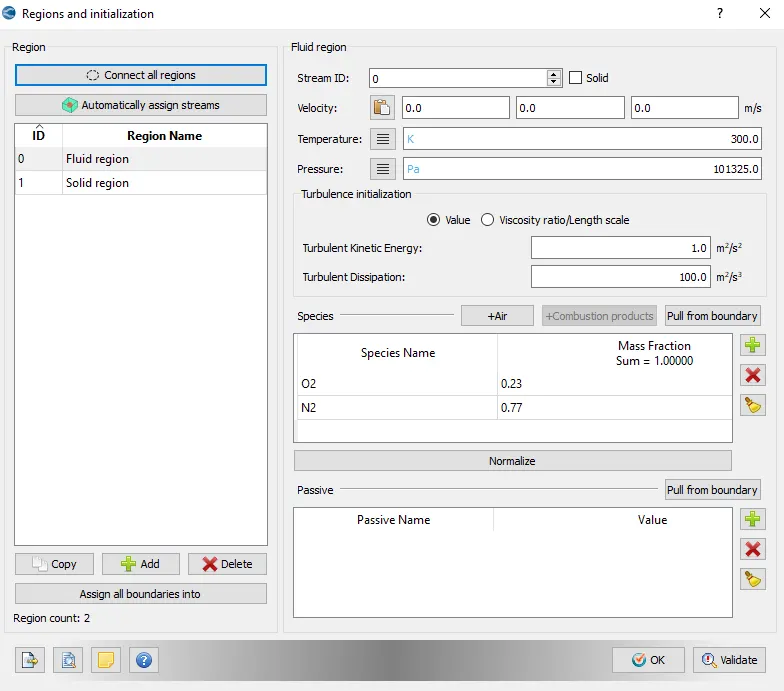
• So far, the front line heading into the liquid realm. Also, for the fluid domain, the boundary must have a wall boundary condition law,and for the reversal region facing the fixed region. Set the Stream ID to 1 in the filled area.
• Set temperature boundary condition to 300K
• Express the boundary conditions as aluminum with a mass fraction of 1.00.
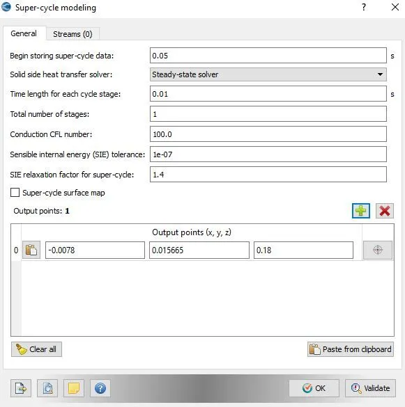
• Next, go to Physics Modeling and enable Turbulence and Super Cycle Modeling. The first option is to set the start time when the super cycle will start saving data. This can be set to any value between 0 and less than or equal to the total simulation time. The solver used for the fixed domain can be steady-state or transient, independent of the solver set in the Run Parameters window.
• The length of time for each cycle determines the interval at which the liquid domain stops and the solid domain dissolves. This interval is considered after the first fluid solver pauses at 1.
• CFL number, SIE tolerance, and relaxation factor are solver parameters specified for solver accuracy and speed. A starting point must be defined in the fixed region so that the solver knows at which point to compute the temperature data. When running the solid domain solver, this point must be specified in the solid domain. Once this value converges, the fluid domain solver continues.
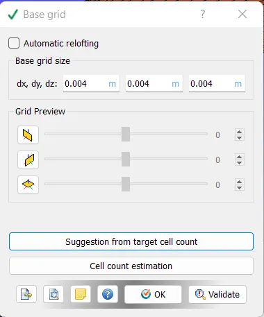
• Run the simulation with 3 base grids of 0.001, 0.002 and 0.004

• Results
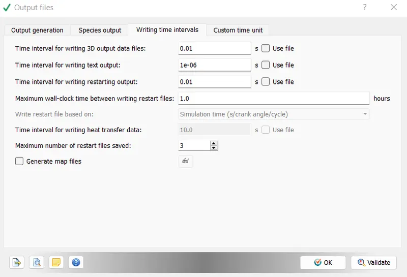
• Supercyle stage interval = 0.01
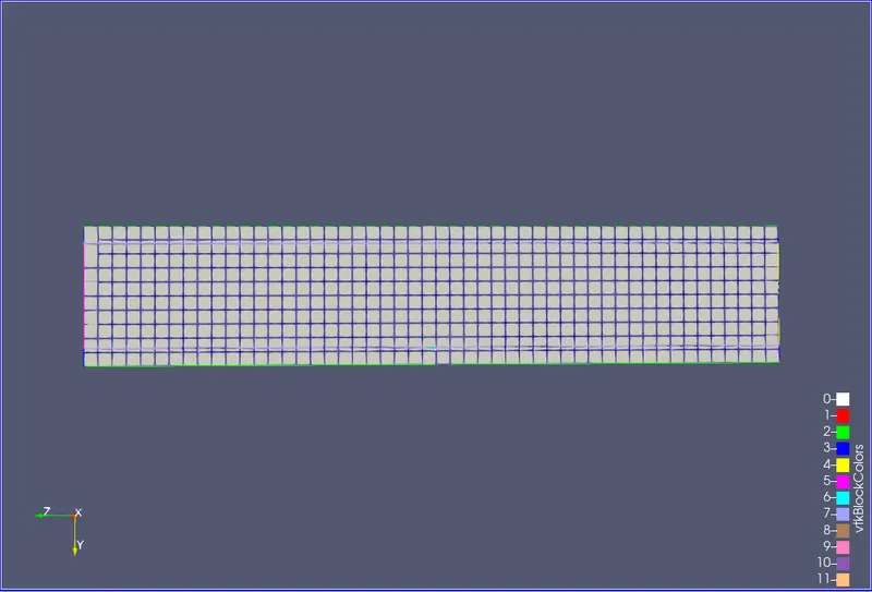
• Grid size = 0.004 m

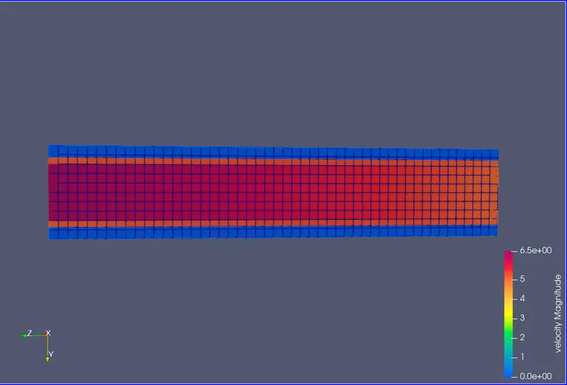
• Velocity contour

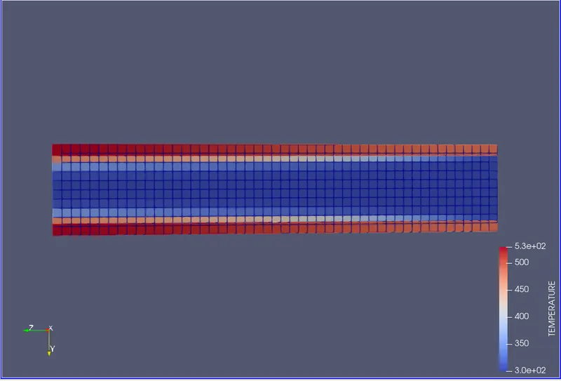
• Temperature contour

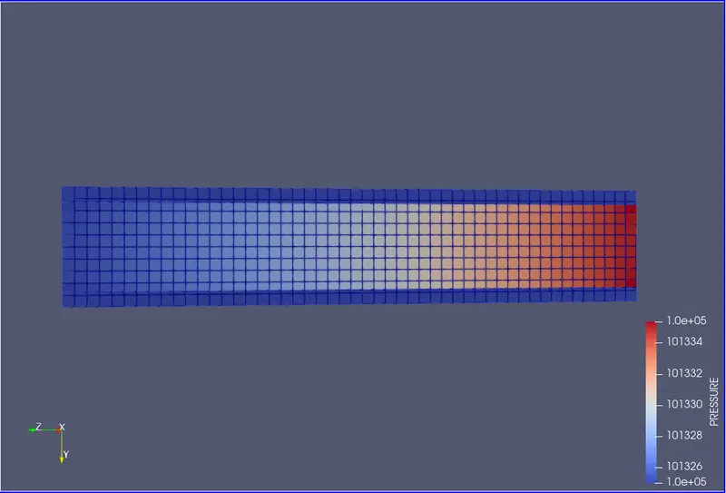
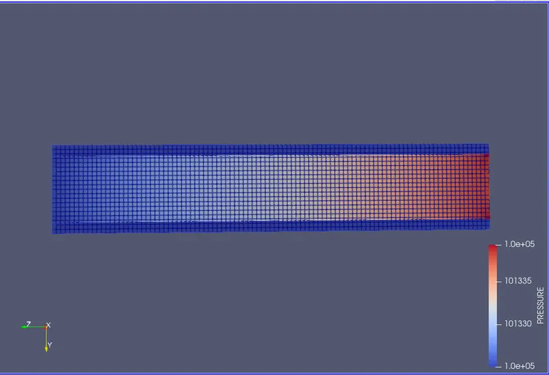
• Pressure contour

• Plots

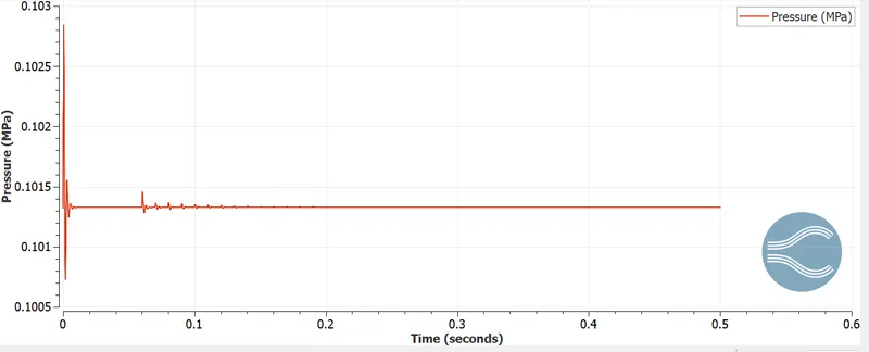
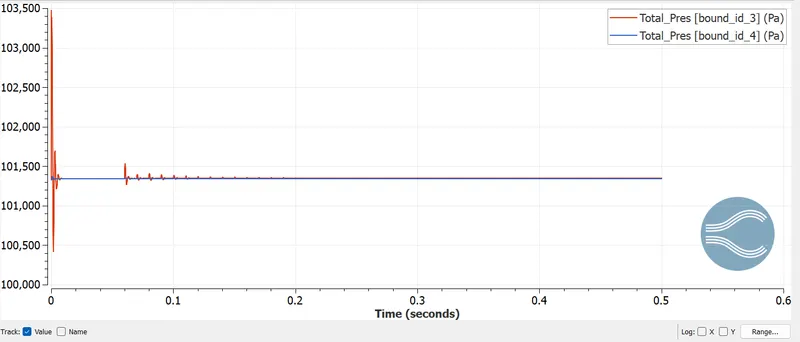
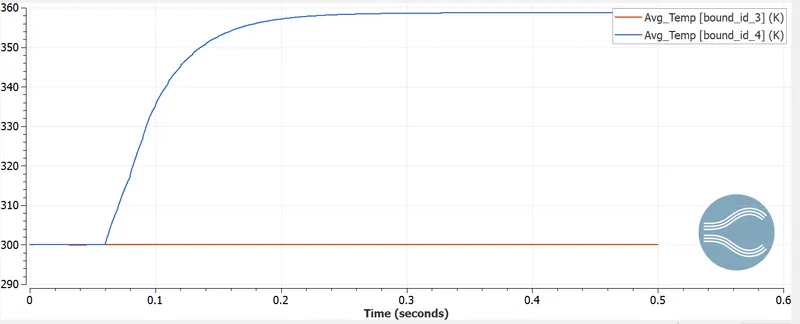
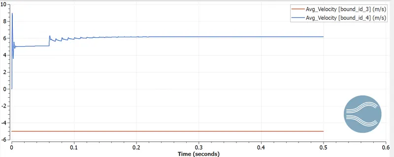
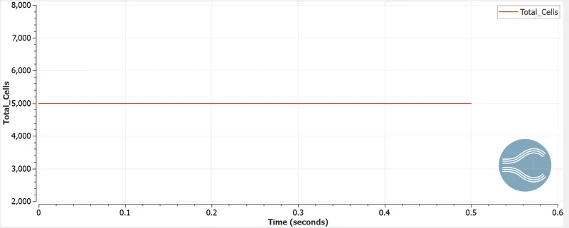
• Solid State Temperature Profile
  As mentioned earlier, applying the steady state solver to the solid state results in a sharp temperature rise at various time intervals. It does not represent the actual temperature profile of the solid, only the steady state temperature. Note that the temperature rise in the solid region is due to additional heat flow in the solid outer wall.
• Fluid Domain Temperature Variation
  The fluid domain flow is simulated with a transient solver and the actual temperature rise in this case is observed. The temperature rise is due to heat transfer from the solid to the liquid.

• Supercyle stage interval = 0.02
• Grid size = 0.003 m

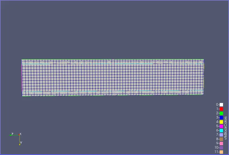
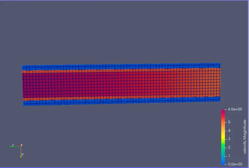
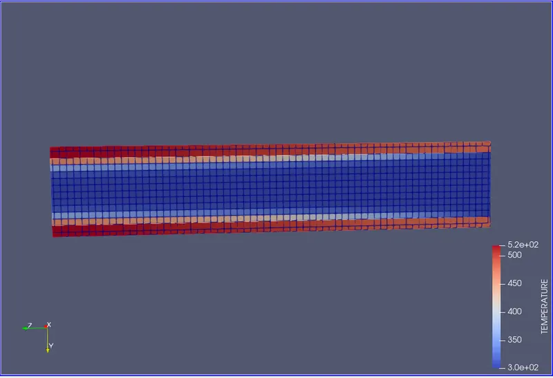
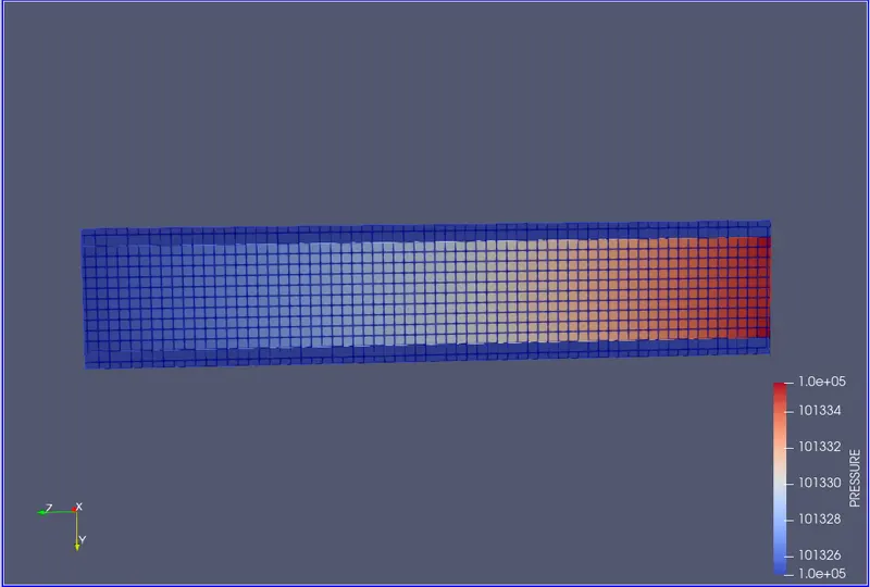
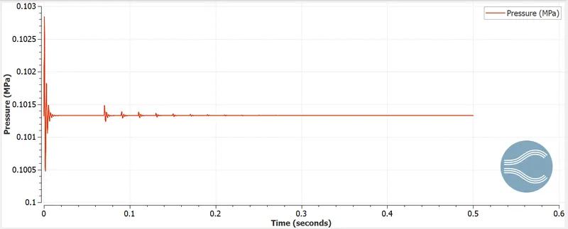
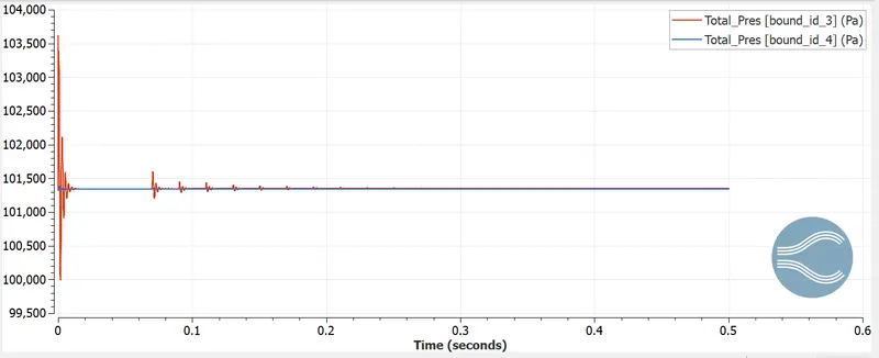
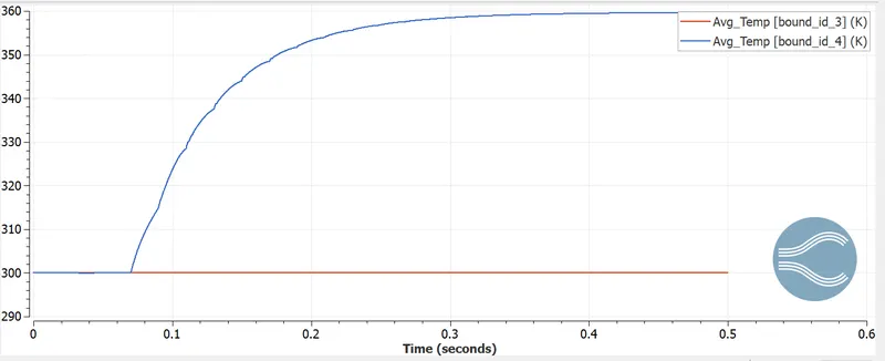
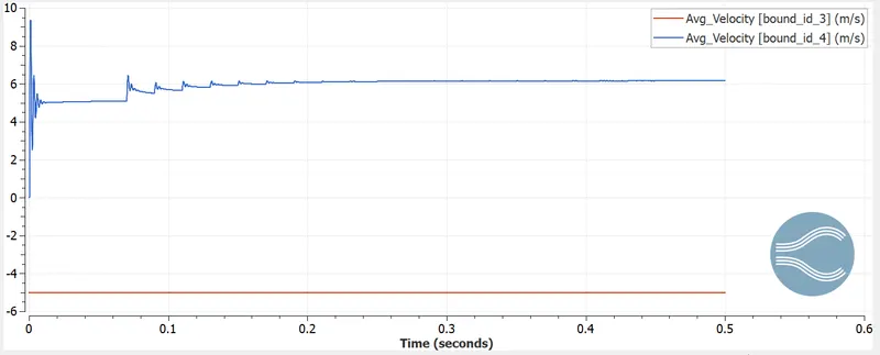
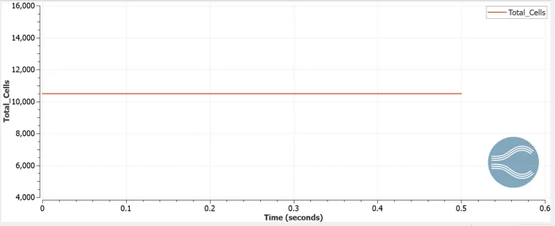
• In this part we performed the grid independency test with 0.002m, 0.003m and 0.004m mesh size. By oberving the above plots we can easily say that at the finer mesh we got the more accurate values of temperature. But at the finer mesh computational effort has been increased.

• Supercyle stage interval = 0.03
• Grid size = 0.002 m

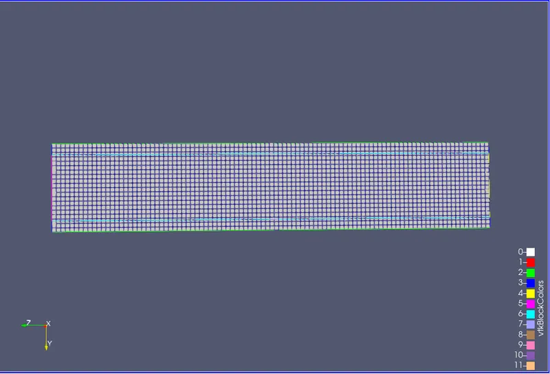
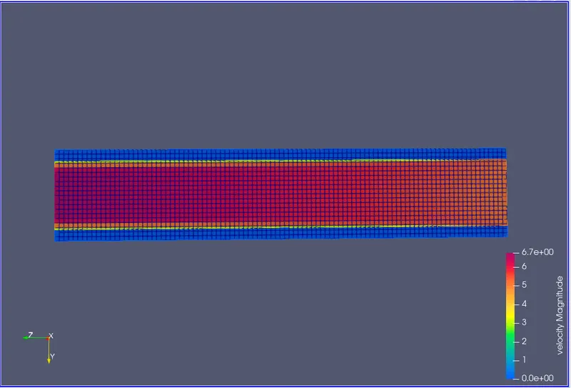
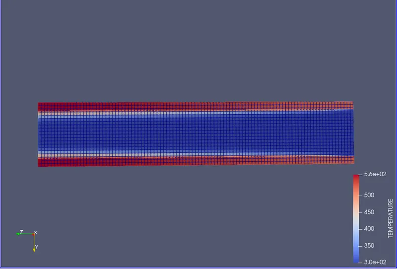
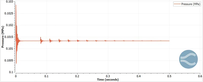
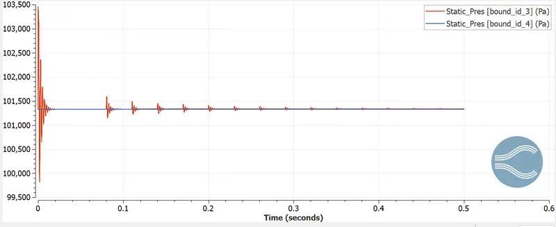
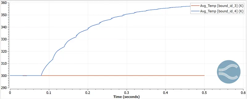
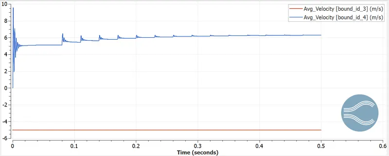
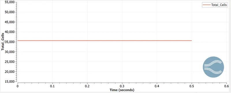
• From the above results, it can be seen that as the air flows through the tube, it is gradually heated until the outlet temperature reaches 380-383 K for various mesh sizes.
• From the Y-plus result, as the mesh gets more refined, we can get the y-plus value, so we get the transition region anyway (for the transition region, the Y+ value is between 10 and 30 must be). While the value of y + is greater than 30, it is a turbulent region.

• Animation links
• https://drive.google.com/drive/folders/1Ynh8kSPyte6DFe3UVXvFn1dQ9zkPQVMC?usp=sharing

• Conclusion
• A transient simulation of conjugate heat transfer for flow through a pipe is run for 0.5 seconds. A heat flux of
  10000 W/m2 is applied to the giant outer wall and an inflow velocity of 3.7 m/s is calculated based on a given Reynolds number of 7000.
• The contours show that the pressure is high at the inlet and gradually decreases at the outlet to the boundary conditions indicated at the outlet.
• The animation shows the temperature variation in the fluid domain due to heat flow applied to the solid outer wall of three different housings with different grid sizes.
• This simulation clearly captures the physics of conjugate heat transfer. A heat flow applied to the outer wall of a solid is shown to pass through the solid domain by conduction and into the liquid domain by convection.