Week 6: Conjugate Heat Transfer Simulation

Objectives:

Air flow simulation through a pipe using conjugate heat transfer analysis & super cycling model.

To perform a grid independence test.

To study the effect of supercycle syage interval.

Introduction:

Conjugate Heat Transfer:-

• Conjuate Heat Transfer correspond with the combination of heat transfer in solid and heat transfer in fluid.
• In solid, conduction often domain whereas in fluid convection usually domain.
• Conjugate heat transfer is observed in many situation. For eg., heat sinks are optimized to combined heat transfer by conduction in the heat sink with the convection in the surrounding field.

Super Cycling Concept

Super cycling is a technique which is used in Converge studio in the case of conjugate heat transfer problems with a solid and liquid regions. Main poblem is that both solvers cannot run at the same speed since solving in fluid domain is much faster owing to the time scale difference for heat transfer in liquids as compared to the solids. This causes problems during the solution given that the solid side solver would not have reached a steady state/convergene in the time the liquid solver does. This is where the concept of super cycling is based.

The basic idea of super cycling is that the solver for the fluid domain is paused until the solver for the solid domain converges. The following steps are involved in performing the super cycling

• Solve the fluid and the solid together with the transient solver. store the instantaneous Heat transfer coefficients and temperature on the interface during process.
• Freeze the fluid solver. Time-averages the Heat transfer coefficients and temperatures and applies them as boundary conditions at the interface.
• Solves the solid temperature until it reaches steady-state.
• Update the solid temp field and unfreezes the fluid solver.
• Repets until the solid temp converges.

Wall Functions and Y+

Gradients of velocity, temperature, etc. close to the wall are large and hence a fine grid resolution is required to accurately resolve the gradients.

Wall Functions are empirical functions that are fitted to the observed behavior close to the wall.

In the turbulent region, we have three layers: the viscous sub-layer, the buffer layer, and the log-law layer. We can use the no-slip condition to resolve the flow in the viscous sub-layer and hence no wall function is required. The wall function can help to resolve the flow in the log-law layer.

We need a method to determine the layer of the flow to s=resolve the flow. This is done by the non-dimensional term Y+, which can be used to understand how coarse or fine our grid is. This can be used to determine if wall functions need to be used or not.

Reynolds number:-

Re =(rho*v*D)/dynamiv viscosity

Geometry:-

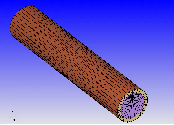
Geometry

Outer Diameter = 0.02 m

Inner Diameter = 0.015 m

Length = 0.2 m

Case Setup:-

Application type:-

• Time based

Material:-

• Gas simulation - Air
• Solid simulation - Aluminium
• Species - on
• Reaction Mechanism - off

Global Transport Parameter:-

• Turbulent Prandtl Number - 0.9
• Turbulent Schemidt Number - 0.78

Simulation Parameter:-

• Solver - Transient State Solver

Simulation time parameter:-

• Start time - 0.0 s
• End time - 0.5 s
• Initial time step - 1e-7 s
• Minimum time step - 1e-7 s
• Maximum time step - 1 s

Region and Initialization:-

1. Fluid Region:-

• Stream ID - 0
• Velocity - 3.66 m/s(z-direction)
• Temperature - 300 K
• Pressure - 101325 Pa
• Turbulent Kinetic Energy - 1 m^2/s^2
• Turbulent Dissipation - 100 m^2/s^3
• Species - Air - O2 - 0.23
• Species - Air - N2 - 0.77

2. Solid Region:-

• Stream ID - 1
• Solid - ON
• Temperature - 300 K
• Pressure - 101325 Pa
• Turbulent Kinetic Energy - 1 m^2/s^2
• Turbulent Dissipation - 100 m^2/s^3
• Species - Aluminium - 1

Boundary Condition:-

• Re = 7000

Diameter of the Fluid Region,

• D = 0.030 m

At an inlet temperature of 300 K, the density and viscosity of air is as follows -

• Density of Air at 300 K,

density = 1.177 kg/m^3

• Viscosity of Air at 300 K,

Dynamic Viscosity = 1.846*10^-5 kg/ms

The inlet velocity can be calculated as

v = (Re*dynamic viscosity)/(density*D)

• v = 3.66 m/s

Physical Model:-

• Turbulance Model: RNG k-Epsilon
• Super-cycle Model:
  
  
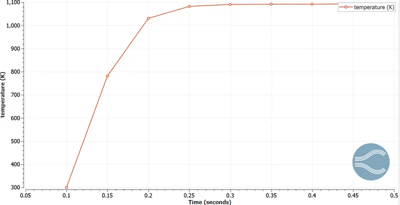
• Begin storing super-cycle data: 0.05 s
• Solid side heat transfer solver: Steady-state solver
• Time Length of each super-cycle stage: 0.05 s
• Total number of stages: 1
• Conduction CFL number: 100
• SIE tolerance: 1e-7
• SIE relaxation Factor: 1.4
• Super-cycle Monitor Point: (0.012933, 0.01179, 0.18)

8. Grid Control:

• Base Grid:
• dx = dy = dz = 0.004 m

9. Output Files:

• Time interval for writing 3-D output files: 0.012 s
• Time interval for writing text output: 1e-6 s
• Time interval for writing restarting output: 0.1 s

OUTPUTS

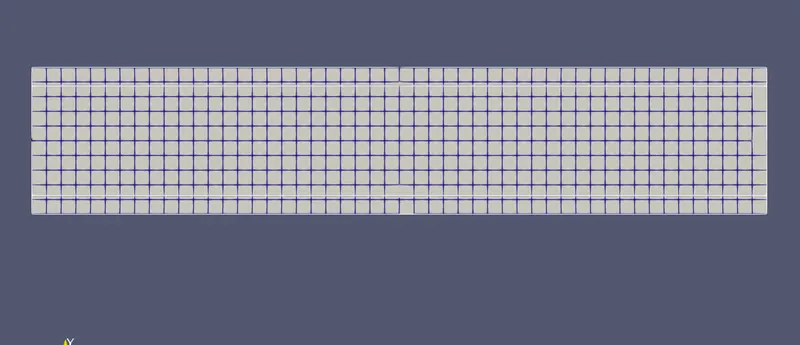
1. Mesh

Mesh

Plots

Super-cycle At The Monitor Point

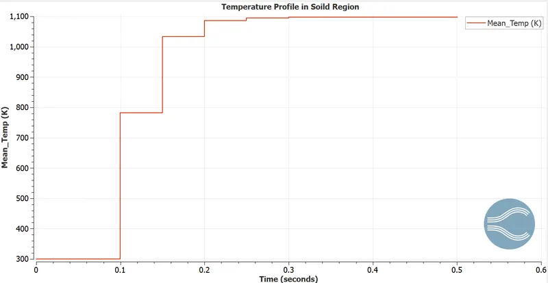
Temp. Profile In the Solid Region

Temp. Profile In the Fluid Region

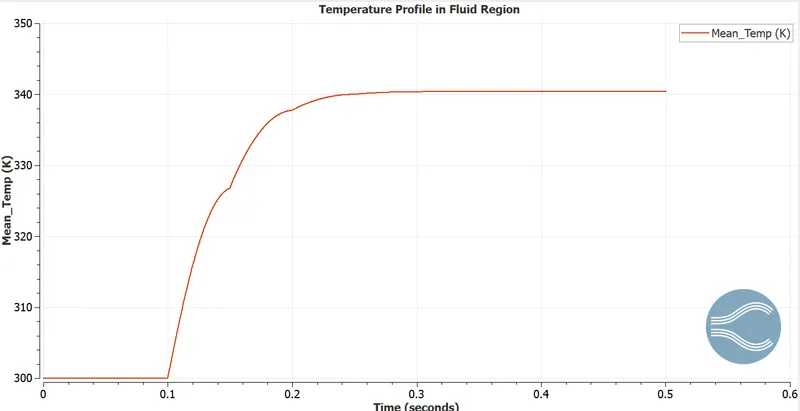
Grid Independence :

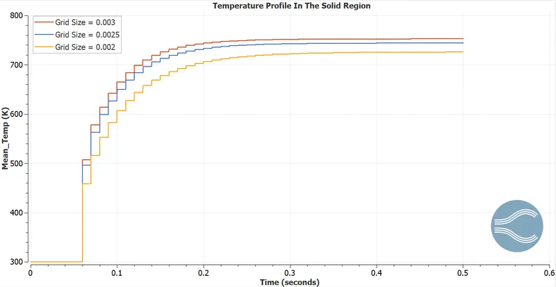
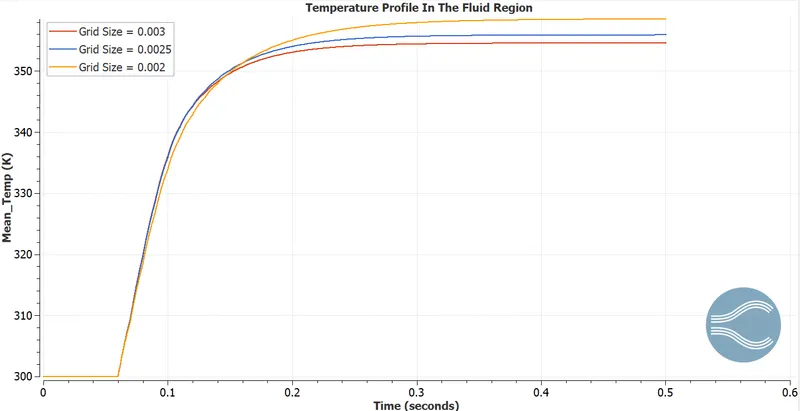
• Case 1: Grid Size = 0.003 m
• Case 2: Grid Size = 0.0025 m
• Case 3: Grid Size = 0.002 m

A. OUTPUTS

1. Mesh

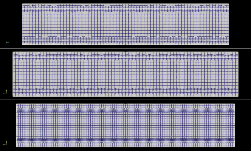
Plots

Temp. Profile In The Solid Region

Temp. Profile In The Fluid Region

VARIATION OF SUPER-CYCLE STAGE INTERVAL

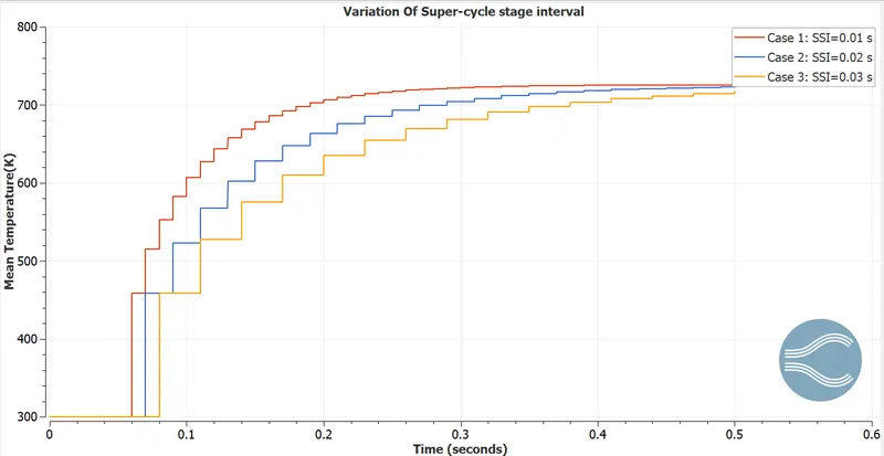
In this part, we shall be varying the time length for each cycle stage that is the super-cycle stage interval, and observe the effects on the mean temperature in the solid region for the entire simulation interval. We shall be considering the following three cases :-

• Case 1: Super-cycle Stage Interval = 0.01 s
• Case 2: Super-cycle Stage Interval = 0.02 s
• Case 3: Super-cycle Stage Interval = 0.03 s

OUTPUT

Temperature contour:

https://drive.google.com/file/d/1GnS5pUGFoxJORUVAtDMb9PljL6fs6Z6q/view?usp=sharing

Y+ Contour

https://drive.google.com/file/d/1bhNS9bSVYLk2bJAsbXBXI5dN9wSpwxdU/view?usp=sharing

Results:

• Increasing the size of the mesh will result in coarse mesh which results in inaccurate results. Alternatively, the mesh can be refined near the boundary to capture the effects accurately.
• The steady-state temperature results do not depict the actual temperature flow in the solid and only the equilibrium temperature. Since we have reduced the super-cycle stage interval, the number of cycles executed to achieve steady-state temperature has increased.

• Decreasing the super-cycle stage interval results in faster convergence of the solution concerning the simulation time.It is better to have a small duration and need the simulation to converge within the given simulation time.

• Decreasing the super-cycle stage interval results in an increase in the number of cycles executed by the solver. This results in more pauses in the fluid solver, which will further increase the computation time of the solution.