Week 6: Conjugate Heat Transfer Simulation

Week 6: Conjugate Heat Transfer Simulation

Aim and Objective:

To simulate, Conjugate Heat Transfer flow through a solid pipe and to understand super cycling.

Baseline configuration:

• To setup a flow simulation through a pipe.
• Inlet Reynolds number should be 7,000
  • Re = (rho*V*D)/(Dynamic viscosity)
• Turbulence modelling - K-Epsilon.
• Supercycling parameters - same as in the video.

Additional 3D outputs

• To add Y+ to your post.in file.

Grid dependence test

• To start with an initial base grid.
• To run grid dependence test on 3 grids and show that the outlet temperature converges to a particular value.

Effect of Supercycle stage interval

• To set Supercycle stage interval to 0.01,0.02 and 0.03
• For these three values, how does the total simulation time compare against the baseline configuration.
• To show the mesh generation using PARAVIEW.

Introduction:

Any matter which is made up of atoms and molecules has the ability to transfer heat. The atoms are in different types of motion at any time. The motion of molecules and atoms is responsible for heat or thermal energy and every matter has this thermal energy. The more the motion of molecules, more will be the heat energy. However, talking about heat transfer, it is nothing but the process of transfer of heat from the high-temperature body to a low temperature one.

According to thermodynamic systems, heat transfer is defined as the movement of heat across the border of the system due to a difference in temperature between the system and its surroundings. Interestingly, the difference in temperature is said to be a ‘potential’ that causes the transfer of heat from one point to another. Besides, heat is also known as flux.

Heat can travel from one place to another in several ways. The different modes of heat transfer include:

• Conduction
• Convection
• Radiation

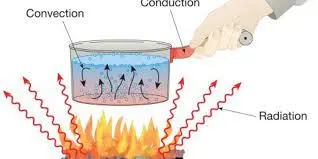
Meanwhile, if the temperature difference exists between the two systems, heat will find a way to transfer from the higher to the lower system.

Conduction is defined as the process in which heat flows from objects with higher temperature to objects with lower temperature. Convection is defined as the movement of fluid molecules from higher temperature regions to lower temperature regions. Thermal radiations are referred to as radiant heat. Thermal radiation is generated by the emission of electromagnetic waves. These waves carry away the energy from the emitting body. Radiation takes place through a vacuum or transparent medium which can be either solid or liquid.

Conjugate Heat Transfer:

Conjugate heat transfer corresponds with the combination of heat transfer in solids and heat transfer in fluids. In solids, conduction often dominates whereas in fluids, convection usually dominates. Conjugate heat transfer is observed in many situations. For example, heat sinks are optimized to combine heat transfer by conduction in the heat sink with the convection in the surrounding fluid. Efficiently combining heat transfer in fluids and solids is the key to designing effective coolers, heaters, or heat exchangers. The fluid usually plays the role of energy carrier on large distances. Forced convection is the most common way to achieve high heat transfer rate. In some applications, the performances are further improved by combining convection with phase change (for example liquid water to vapour phase change).

Heat sinks are usually made of metal with high thermal conductivity (e.g. copper or aluminum). They dissipate heat by increasing the exchange area between the solid part and the surrounding fluid. Temperature field in a power supply unit is cooling due to an air flow generated by an extracting fan and a perforated grille. Two aluminum fins are used to increase the exchange area between the flow and the electronic components.

Time Control for Conjugate Heat Transfer Modelling:

There are three approaches. The first approach is by using transient approach, where we are solving a simulation from a start time to the end time and we are dividing this entire range into multiple time steps and each time step is being solved accurately, which is the most accurate way of running the simulation, but this can be very slow because if we consider a solid, the time scale associated with the heat transfer can be much higher than the time scale associated with the fluid flow. In this case we might use second approach that is steady state approach if we really don't care about the time history of temperature and it will result in the final temperature distribution very quickly. This approach is highly desirable in such cases when we have a steady state flow pattern.

Super Cycling Approach:

The final approach is the super cycling approach. This is recommended for the simulations with combustion. In this approach we are solving the fluid part completely transient, in which we will basically run the steady state simulation on the solid part time to time, so that we will get results in a quicker way. Transient solver solves the fluid and solid part together for a particular time, once the time is up, we average the gas temperature and heat transfer co-efficient near the walls and then we will consider the averages values and run the steady state simulation on the solid side and when we run the steady state simulation, the fluid solver is frozen until the solid part converges. So from this way we can get the temporal accuracy on the fluid side and also the temperature distribution in a quick way. This process is going to work very well if we are interested only in final temperature distribution.

This process of super cycling makes sure that the final temperature is accurate as we are solving the gas phase transiently.

The following steps are involved in performing the super cycling approach:

• Solves the fluid and solid parts together with transient solver.
• Freezes the fluid solver.
• Solves the solid temperature until it reaches steady state.
• Updates the solid temperature field and unfreezes the fluid solver.
• Repeats until the solid temperature converges.

Geometry Setup:

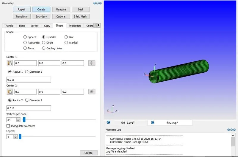
• The pipe is created using the following steps.

Create --> Shape --> Cylinder --> Enter the value in Center 1 and Center 2 --> Enter the radius value = 0.015 --> Create.

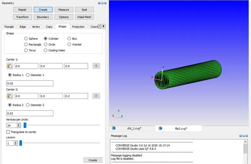
Similarly another cylinder with the radius of 0.02 m is created.

• After the creation of these cylinders a diagnosis check has been done. In that we found an error in intersections. In order to correct this error the following steps have been done.

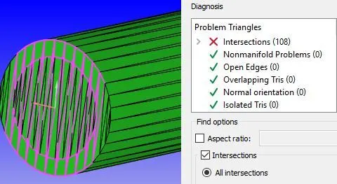
• To avoid the intersections in the geometry, deleting the front two faces and back two faces of the geometry is done.
• Repair --> Delete --> Triangle --> use By angle as entity --> using cursor pick --> selecting triangles on larger diameter circular face --> Apply.

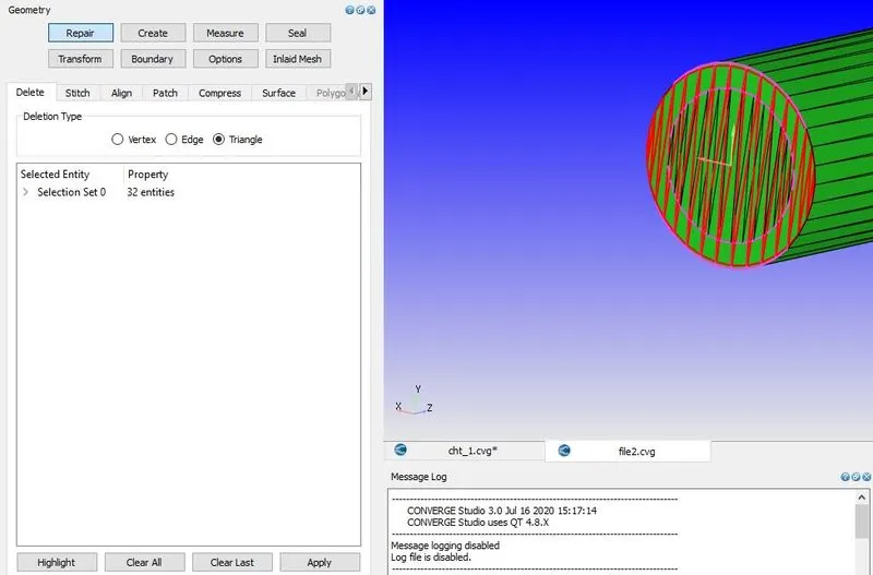
• And the same procedure is done for deleting the smaller diameter circular face.

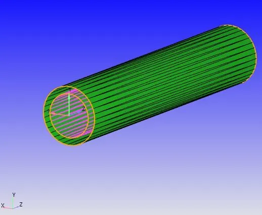
• To create a flow passage for fluid and to separate the fluid body and solid body a thickness is provided by creating triangles. This will also help in assigning the inlet and outlet boundary.
• Create --> Triangle --> Loft edges --> Edge as an entity --> By open edge --> Selecting the larger diameter edge as the first set of edge and then selecting the smaller diameter as the second set of edge --> Apply.

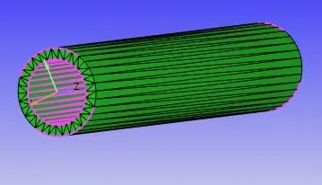
• In converge every part of geometry is assumed to be a triangle. Selecting triangles and grouped to assign to specific boundaries. In the next step the boundaries are flagged with names.

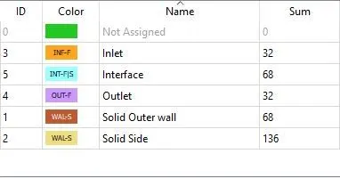
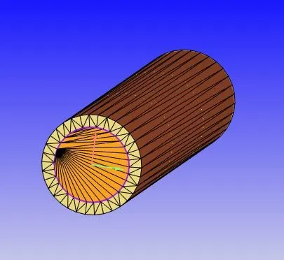
• The non-manifold problems occur due to the presence of three surfaces of a triangular element in contact with each other which are not recommended in ordinary simulations but are unavoidable in CHT analysis. After assigning the triangles to interface boundary, there are no manifold problems present. The interface boundary region (highlighted in blue colour) is as follows:

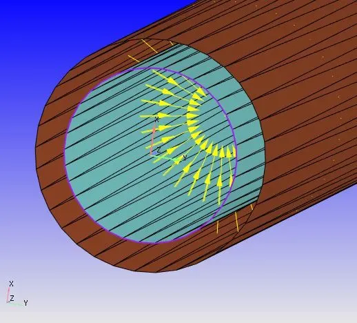
• Every geometry have a normal vector, it points perpendicular to it. In this project the normals are assigned in the way that the fluid flow is internal as mentioned in the above figure.
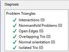
• Diagnosis check after the geometry is setup.

Case Setup:

• The application type is fixed with time based.
• Then click on Materials which is present in the right side of the window that is case setup tree and select the Predefined mixtures as Air and since we are doing both fluid and solid simulation check the "Solid Simulation" checkbox and "Species" checkbox. And then uncheck the "Reaction Mechanism" checkbox.
• Click on the Gas simulation and Global Transport parameter and retain the same values. Click on the Solid simulation, add the predefined solids to be Aluminium.
• Click on Species and then add O2 and N2 in Gas and Aluminium in Solid.
• Click on Run Parameters and under the solver tab choose the solver as Transient. Set the simulation mode to Full Hydrodynamic and the gas flow solver as compressible.
• Then under "Misc" tab check the use shared memory boxes.
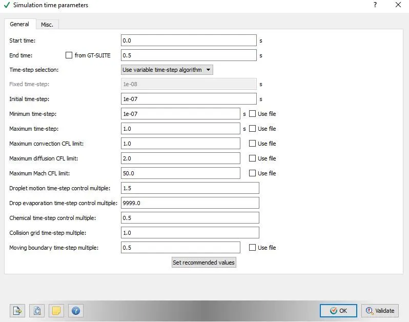
• In the Simulation time parameter do the following changes.

• In the solver parameter choose the pressure based solver and retain the same values.
• Then under Regions and Initialisations, create two regions named Fluid and Solid.
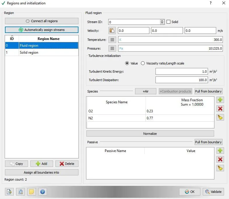
• In the fluid region set the stream id as 0 and velocity condition as (0, 0, 0). Temperature initial condition as 300K and pressure condition as 101325 pa. Add the species to be air.

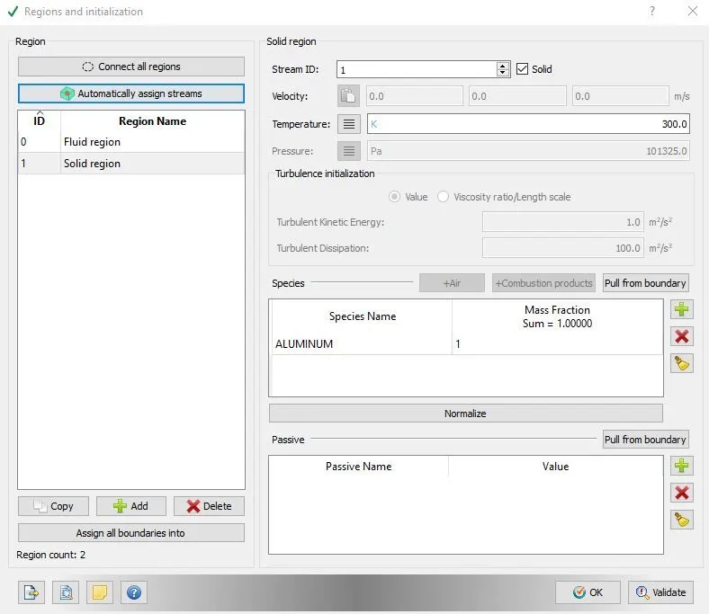
• In the solid region set the stream-id as 1. Set the temperature boundary condition as 300K. Specify the boundary condition as Aluminum with a mass fraction of 1.0

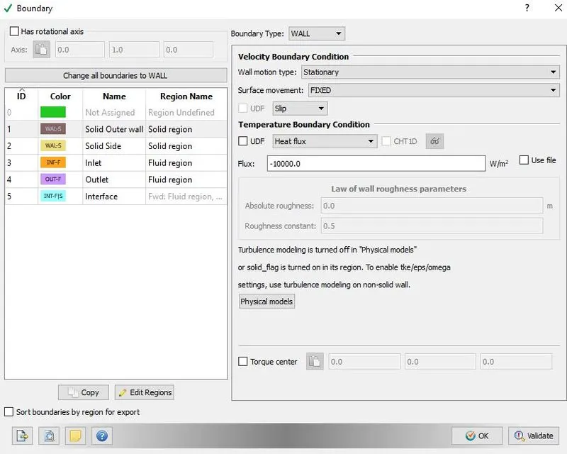
• Then under Boundary Conditions under select the "Solid Outer wall" region and set the boundary type as "Wall" and set the value for Heat Flux as -10000 in the temperature boundary condition. Select the region as Solid region.

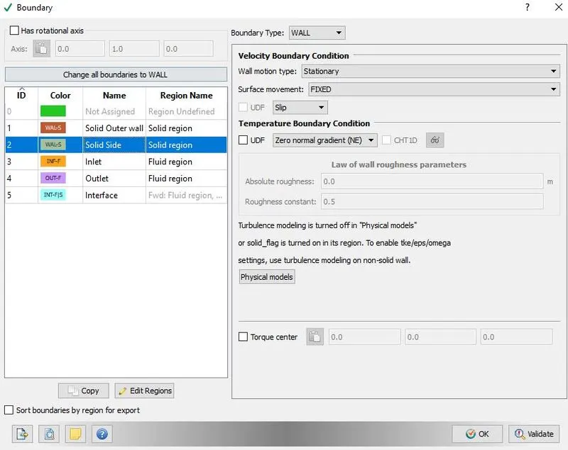
• In the Solid Side boundary region, choose the boundary type as Wall. Set the Velocity Boundary condition as Slip. Set the temperature boundary condition as a zero normal gradient. Select the region as Solid region.

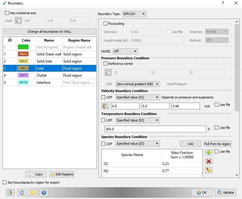
• Then under Inlet boundary region, we are choosing the boundary type to be Inflow condition. Choose the zero normal gradient in the Pressure Boundary Condition. Select the specified value in the velocity boundary condition and enter the velocity to be 3.71 m/s in the Z-direction. Select the specified value in the temperature boundary condition and enter the temperature value to be 300K. Add the species in the Species Boundary Condition. Select the region as Fluid region.

• Calculating the Velocity at inlet based on Reynolds number:

  Given:

  Reynolds number = 7000

  Inner diameter (fluid region diameter) = 0.03 m

  Properties of air at 1 atm pressure and 300 K.

  Density of air at 300K and 1 atm = 1.177 `(kg)/m^3` (`rho`)

  Dynamic Viscosity = 0.00001846 `(kg)/(ms)` (`mu`)

  Reynolds number is calculated using the following formula,

  `Re= (rho*V* D)/mu`

  Therefore velocity is calculated by,

  `V= (Re*mu)/(rho*D)`

  `V= (7000*0.00001846)/(1.177*0.03)`

  V= 3.66 m/s.

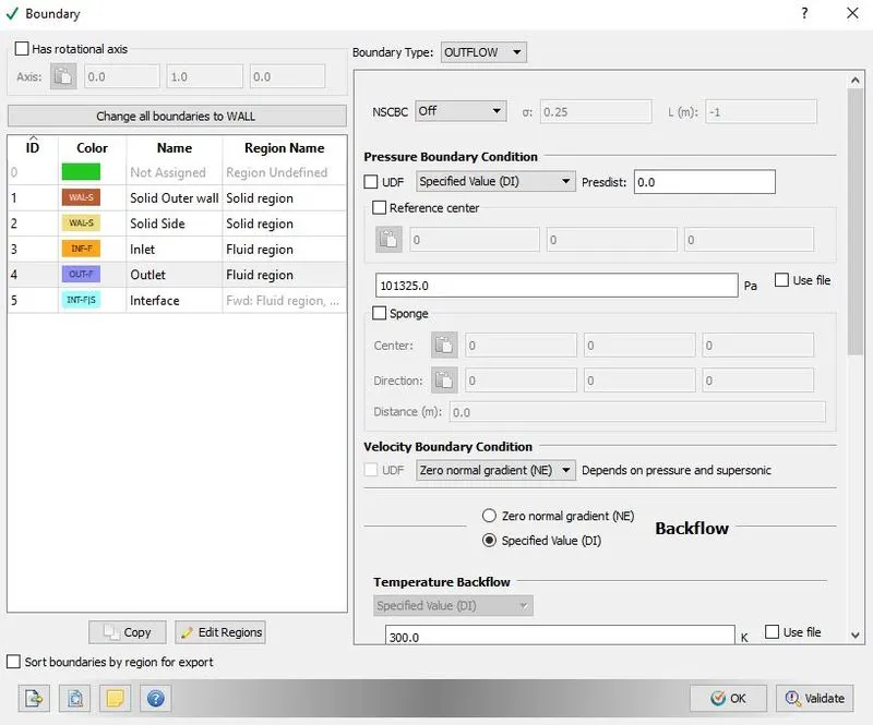
• Then under Outlet boundary region, we are choosing the boundary type to be Outflow condition. Choose the specified value in the Pressure Boundary Condition and enter the values of pressure to be 101325.0 pa. Select the specified value in the temperature boundary condition and enter the temperature value to be 300K. Add the species in the Species Boundary Condition. Select the region as Fluid region.

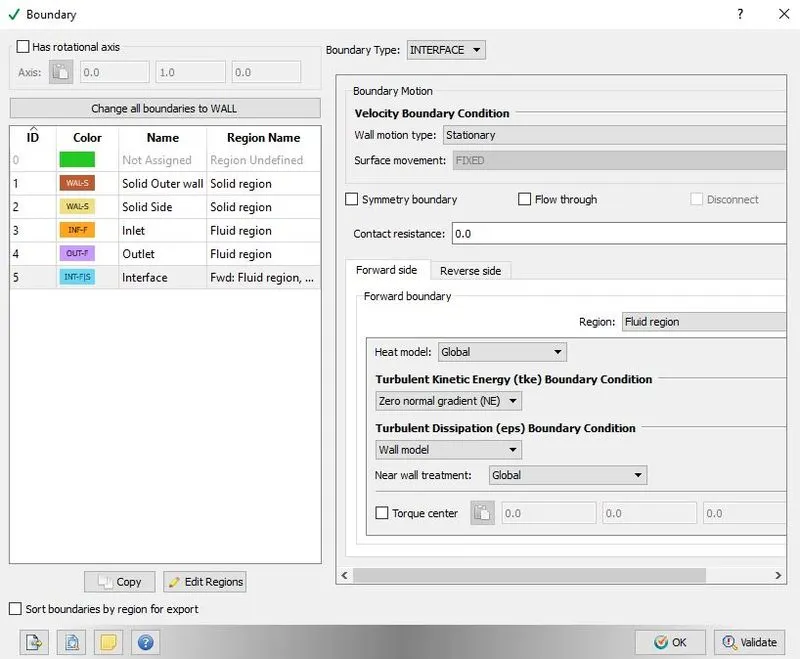
• Then under Interface boundary region, we are choosing the boundary type to be INTERFACE condition. Select the wall motion type as Stationary. This boundary is the interface between solid and fluid regions, so two different boundaries are set. In the Forward side set the velocity boundary condition as Law of Wall and set the temperature boundary condition as Law of wall.

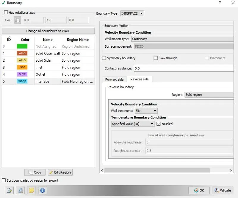
• In the Reverse side set the region to be solid. Set the velocity boundary condition as Slip and temperature boundary condition as specified value.

• Then under the physical models check the Turbulence and Super cycling modelling and set with Reynolds Averaged Navier-Stokes (RANS) and set the turbulence model with RNG K-epsilon.

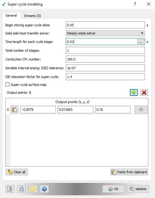
• The first option is to set the initial time at which the super-cycle begins storing data. This can be set from 0 to any value less than or equal to the total simulation time. The solvers used for the solid region can be a steady or transient solver that is independent of the solver set in the run parameters window and can be steady or transient. The time length to each cycle determines the intervals at which the fluid domain is paused and the solid domain solved for. This interval is taken into account after the initial pause of the fluid solver at 1.The CFL number, SIE tolerance and relaxation factors are solver parameters that are given for the purpose of accuracy and speed of the solver. An output point must be defined in the solid region to let the solver know at which the temperature data must be calculated. This point must be given in the solid domain as the solver runs for the solid domain and once this value converges, the fluid domain solver is continued.

Grid Control:

Kinematic Viscosity `V=mu/rho=0.00001846/1.177`

`V=0.000015684 m^2/s`

Skin friction drag co-efficient `C_f=0.0576*Re^(-1/5)=0.0576*(7000)^(-1/5)`

`C_f=0.00980399`

Wall Shear Stress `T_w=C_f*(rho.V^2)/2=0.00980399*(1.177-(3.66)^2)/2`

`T_w=0.077287898N/m^2`

Frictional Velocity `u_t=root2(T_w/rho)=0.256310311m/s`

Assuming the desired y+ to be 32.

Then the first cell centre to boundary distance `y=y_+ * V/u_t = 32*0.000015684/0.256310311`

y=0.001958126 m

Cell Size = 2 times of y times 1000 = 3.9162 mm

Which is 4mm approximately.

Then in the Grid Control parameter --> Base Grid --> Enter the size of the grid.

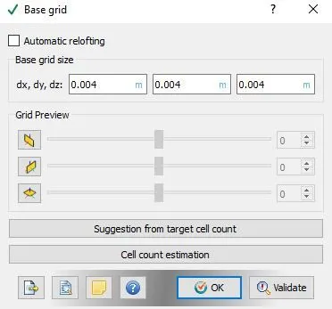
Changing the value of the grid size for Grid Dependence Test.

• Then under Output/Post-Processing --> Post Variable Selection --> retain the same values. Add the y+ turbulence model under Combustion/Turbulence.
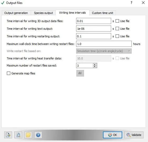
• Then under the Output files --> Writing time intervals --> set the time interval for writing 3D output data files and time interval for writing restarting output.

• Then export all the input files to the desired location.
• Then use CYGWIN to execute the CFD solver.
• Then with the help of Converge CFD the post converting the output files to Paraview format is done.
• Paraview is used for Post processing the results.

Results:

Grid Dependence test:

Case 1:

Grid size = 0.004 m

Super cycling interval = 0.05 s

Case 2:

Grid size = 0.003 m

Super cycling interval = 0.05 s

Case 3:

Grid size = 0.002 m

Super cycling interval = 0.05 s

Grid Dependence test:

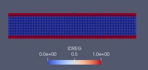
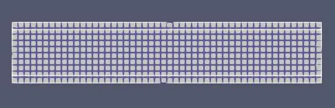
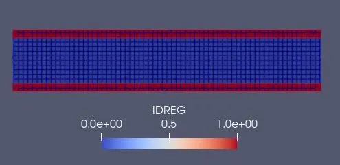
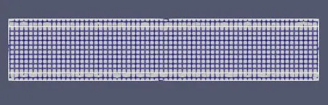
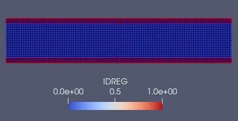
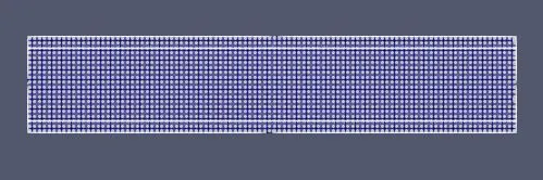
Mesh:

Case 1:

Grid size = 0.004 m

Case 2:

Grid size = 0.003 m

Case 3:

Grid size = 0.002 m

Pressure Contour:

Case 1:

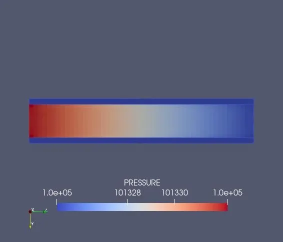
Case 2:

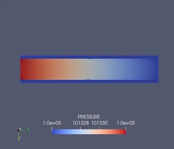
Case 3:

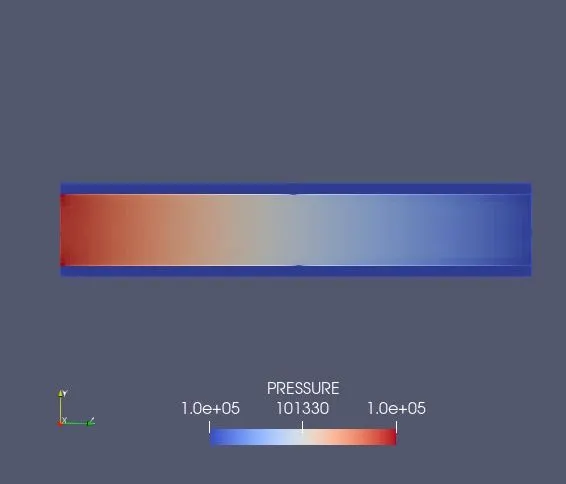
Velocity Contour:

Case 1:

Case 2:

Case 3:

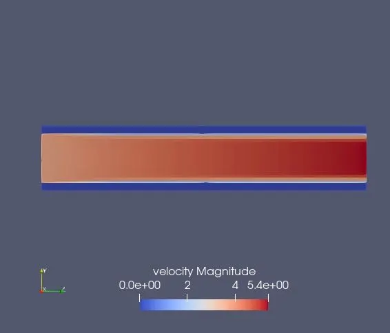
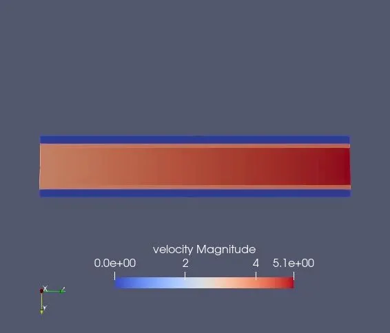
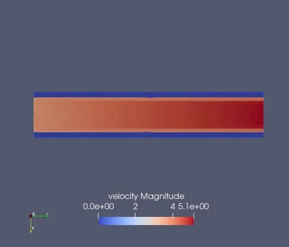
Using finer mesh have given precise details of changes in flow pattern in earlier problems. Similarly, in this case it can be observed that as mesh size is reduced to 0.002 m, finer flow of contour of temperature, velocity and y+ boundary values are obtained.

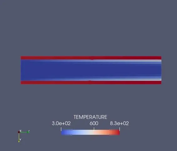
Temperature Contour:

Case 1:

Case 2:

Case 3:

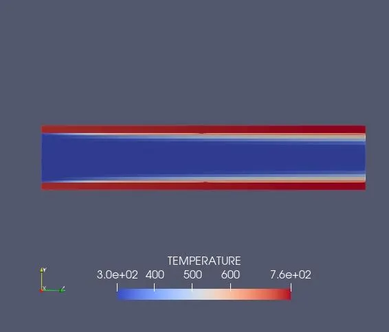
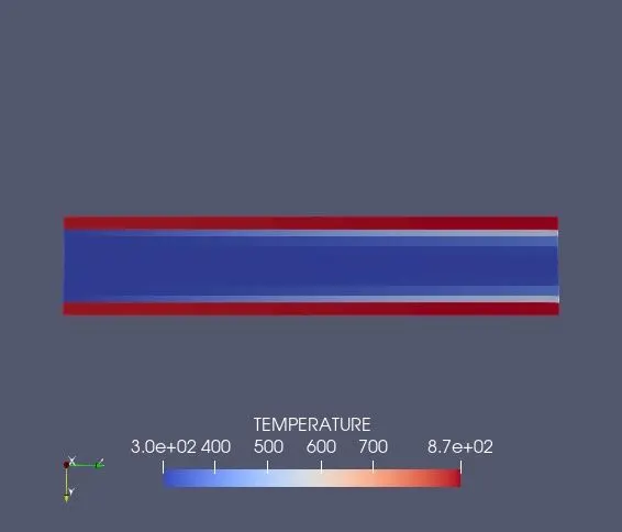
From the above temperature contour for all 3 grids, it is observed near the outlet side there are clear difference in all the three grids. With more refinement, the outer temperature has converged slightly different values. Even the coloured profile observed in the base grid just below the solid region is less dense but as moved to grid 0.003 m it is more shaper and even more at the finer grid 0.002 m.

Animation video:

Velocity:

Case 1: https://youtu.be/hLj7MFOwB8w

Case 2: https://youtu.be/7GvrmWPd5iE

Case 3: https://youtu.be/9Pll2owU4nQ

Pressure:

Case 1: https://youtu.be/nqJvoc3Wy2Y

Case 2: https://youtu.be/CdobHc3X7tc

Case 3: https://youtu.be/uIG6ilrh9Q8

Temperature:

Case 1: https://youtu.be/_4Ulmv9WMMI

Case 2: https://youtu.be/EuBFubc-ZF0

Case 3: https://youtu.be/uGfWpqUVjbg

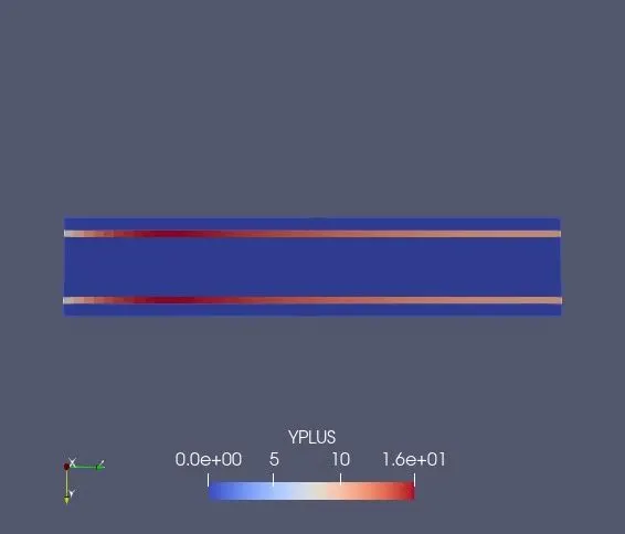
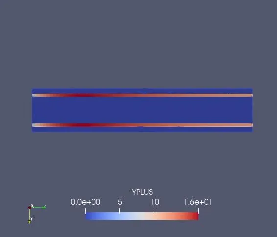
Y+ Contour:

Case 1:

Case 2:

Case 3:

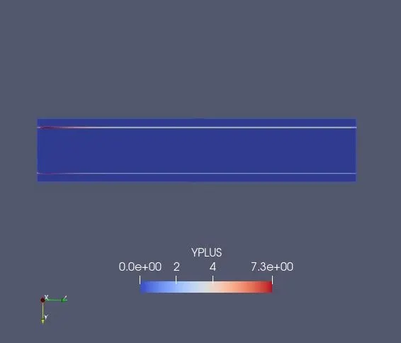
Near the wall regions, it is well known that the mesh size should be small enough because near wall regions have large gradients in the solution variables. Momentum and other scalar transports occur more vigorously. The wall y+ is a non-dimensional distance similar to local Reynolds number, often used in computational fluid dynamics to describe how coarse or fine a mesh is for a particular flow. It is the ratio between the turbulent and laminar influences in a cell.

Accurate presentation of the flow in the near-wall region determines the successful prediction of wall-bounded turbulent flows. However we have a problem when the y+ lies in the range between 10 and 30. Here, it is not easy to predict the solution in transition region. The best practice here is to go finer to the laminar region and just use the no-slip condition or another idea would be to use a coarser grid and go for a wall function instead.

Temperature plots:

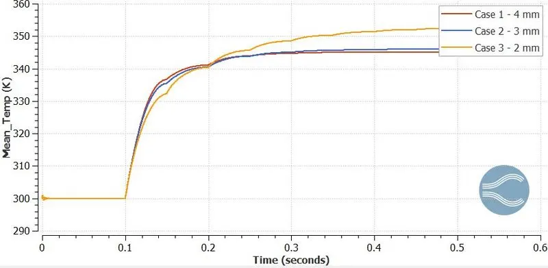
The thermo_region0.out represents the temperature in fluid region adn thermo_region1.out represents the temperature in the solid region.

Fluid region plot for all the 3 cases:

Solid region plot for all the 3 cases:

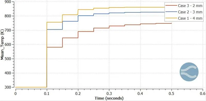
The above plots show the mean outlet fluid temperature and solid temperature for three different grid size values. Although they do not converge to the same specific value, they all are around a decent margin. It is clear that the fluid temperature is around 350 K and the solid temperature is around 850 K. It can be observed that the temperature change is quite significant and is grid dependent. Choosing finer mesh would provide us with some reliable results but with a current computational source mesh size of 0.002 m is more reliable and can be concluded that mesh size smaller than 2 mm can show a grid independent nature. It can be observed that the coarser mesh converges at faster rate but a finer mesh provides accurate results. We could observe that for finer mesh the solid region mean temperature is low, whereas the fluid region's mean temperature is higher for a finer mesh. Here the temperatures are sensitive to changes in mesh grids and hence we can reduce the mesh size further to obtain high level accuracy until these results become independent of the mesh.

Y+ data:

Y+ is a non-dimensional length scale that is normalised using wall shear stress. Since each turbulence model simulates the boundary condition, so the value of y+ is an important parameter to predict the flow field of the boundary layer. The turbulent boundary layer consists of 3 layer wherein different relations are observed between the average velocity and this non dimensional distance y+.

Max y+ values for different mesh size according to the above case:

Case 1:

Grid size : 0.004 m

y+ value: 16

Case 2:

Grid size: 0.003 m

y+ value: 16

Case 3:

Grid size: 0.002 m

y+ value: 7.3

Effect of Supercycle stage interval:

Case 4:

Grid size = 0.003 m

Super cycling interval = 0.01 s

Case 5:

Grid size = 0.003 m

Super cycling interval = 0.02 s

Case 6:

Grid size = 0.003 m

Super cycling interval = 0.03 s

The mesh grid size is fixed with 0.003 m and different supercycle stage interval values of 0.01, 0.02 and 0.03 are compared.

Temperature plots:

The thermo_region0.out represents the temperature in fluid region and thermo_region1.out represents the temperature in the solid region.

Fluid region plot for all the 3 cases:

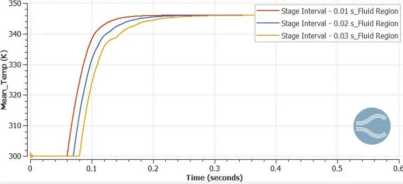
Fluid region plot for all the 3 cases:

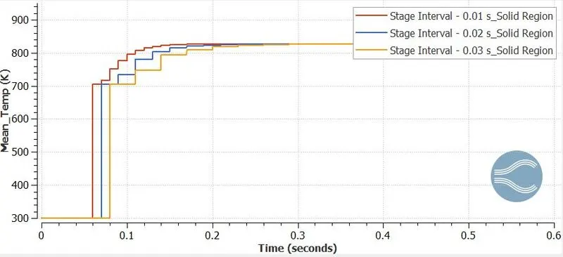
It was observed that when the super cycle values are reduces it takes a lot of time for computing. The higher the super cycle value the lower the time taken for computing. The above temperature curve attains convergence early at the lowest value of super cycle amongst the values given. This could be employed for finer mesh where convergence delays to attain it at a faster rate. Hence, thereby the end time could be shortened which could save the computation time.

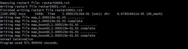
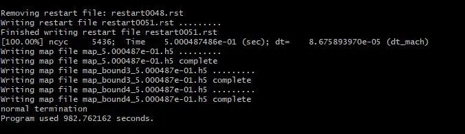
Computational Time for different Super Cycle stage intervals:

Case 1 (Super cycle stage interval - 0.01 s):

Case 2 (Super cycle stage interval - 0.02 s):

Case 3 (Super cycle stage interval - 0.03 s):

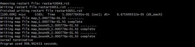
No major difference is observed in simulation time. The size of the mesh is considered as 0.003 m for all super cycle stage interval comparison. Simulation time gets modified only if the grid size of the geometry is changed.

Conclusion:

• The numerical analysis for CHT simulation of a pipe flow model using different super cycling stage intervals with RKE turbulence model based on the governing flow conditions in Converge studio and executed using Cygwin64 terminal was well understood.
• We have performed the grid dependence test with 0.004, 0.003, 0.002 m. From the above plots, we could observe that as the mesh gets finer, the accuracy in the results increases. But when the mesh goes more finer the computational cost and time have been increased.
• Supercycle stage interval is required only if there is solid and fluid contact occurs.
• From the usage of different super cycle intervals we could observe that the lower value of super cycle stage interval, the convergence is achieved faster. We could understand that in this approach we are solving the fluid part completely transient, in which we will basically run the steady state simulation on the solid part time to time, so that we will get results in a quicker way.
• Transient solver solves the fluid and solid part together for a particular time, once the time is up, we average the gas temperature and heat transfer co-efficient near the walls and then we will consider the averages values and run the steady state simulation on the solid side and when we run the steady state simulation, the fluid solver is frozen until the solid part converges. So from this way we can get the temporal accuracy on the fluid side and also the temperature distribution in a quick way.
• From the grid dependency test it can be concluded that as the mesh size reduces the y+ value reduces. Moreover, it is found that the value of mean temperature varies as the mesh size changes. Mesh size can be reduced to increase accuracy until the flow contour become independent of it.