Conjugate Heat Transfer Simulation of heating of a flowing fluid in a pipe

I. Aim: Conjugate heat transfer (CHT) simulation of heating of a flowing fluid in a pipe using Converge CFD.

II. Introduction:

Conjugate heat transfer (CHT) is the heat transfer mechanism occurring at a solid-fluid interface. This type of heat transfer includes both convection (fluid side) and conductive (solid side) heat transfer. The fluid side convection may be natural convection or due to forced convection.

The common examples of CHT are heat transfer between different fluids through heat exchangers, cooling of automobile engines with fins, heat sink applications in electronic equipment, electric motor cooling, and battery thermal management in Electric vehicles, etc. Forced convection on the fluid side plays an important role in achieving high heat transfer rates between the solid surface and the fluids.

Designing the optimum heat transfer interface between the solid surface and the heat transfer fluid plays an important role in keeping the electronic equipment, automobile engines, Electric vehicles, Industrial machinery at their operating temperatures, and better heat transfer in heat exchangers to maximize the performance efficiencies.

CHT analysis comes into the picture in designing the optimum heat transfer model for the above applications. Particularly, numerical CHT analysis using CFD plays an important role to design better heat transfer mechanisms. Using CHT analysis the optimum material and geometry for the solids as well as the flow rates and fluid properties can be realized for each application. The CHT analysis in CFD solves the convection physics on the fluid side and conduction physics on the solid side.

Problem Statement: Perform 3D transient thermal analysis of heating of a fluid flowing through a pipe. The case setup is done using ConvergeCFD and simulation is run in the CYGWIN terminal. Further, post-processing is done using Converge CFD and ParaView.

III Objectives:

• Setup a flow simulation through a pipe
• Inlet Reynolds number should be 7,000
  • Re = (rho*V*D)/(Dynamic viscosity)
• Turbulence modeling - K-Epsilon

Grid dependence test

• Start with an initial base grid
• Run grid dependence test on 3 grids and show that the outlet temperature converges to a particular value

Effect of supercycle stage interval

• Set supercycle stage interval to 0.01,0.02 and 0.03
• For these three values, how does the total simulation time compare against the baseline configuration

IV. Solving & Modelling approach:

3D transient CHT analysis of heating of a fluid in a pipe case is set up in ConvergeCFD and then the solution is run in CYGWIN terminal. Air is used as the fluid flowing through the channel (77% N2 and 23%O2). Postprocessing is done using ConvergeCFD and ParaView. Three meshes are used to check the effect of cell size on the results. Further, the effect of super-cycling stage interval on the heat transfer and temperature distribution is studied.

1. Geometry/Domain:

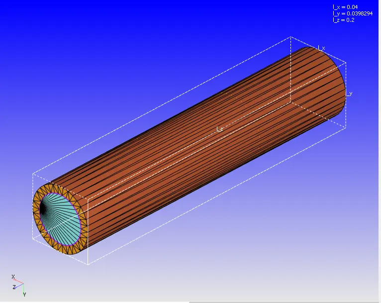
A 3D solid geometry of the typical pipe is created in ConvergeCFD. The following figure shows the pipe geometry. In Converge CFD triangles are the basic building blocks. Hence the surfaces of the pipe are a combination of triangles. The dimensions of the pipe are as follows:

Inner diameter = 0.03 m

Outer diameter = 0.04 m

Pipe length = 0.2 m

2. Boundary Flagging:

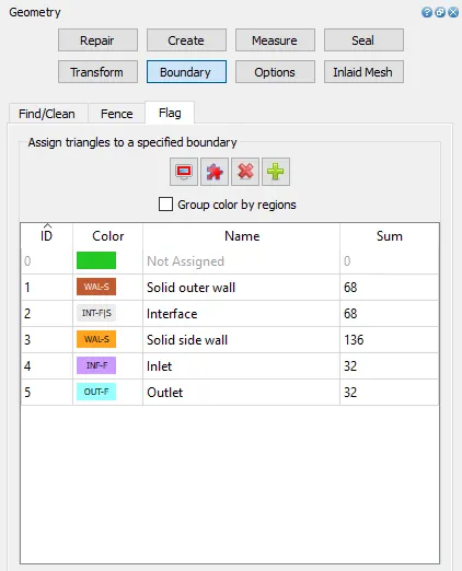
The boundary zones in ConvergeCFD are created by flagging boundaries. This is done by grouping a set of surface triangles into boundary flags in the boundary tab as shown below:

3. Case setup:

After assigning boundary zones as mentioned above, the solution case setup is to be done. ConvergeCFD has a dedicated menu to completely set up the solution. Details are as follows:

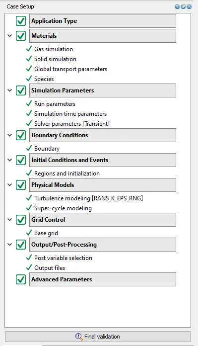
-In the application type option, Time-based is selected.

- The materials option are selected as shown in below images:

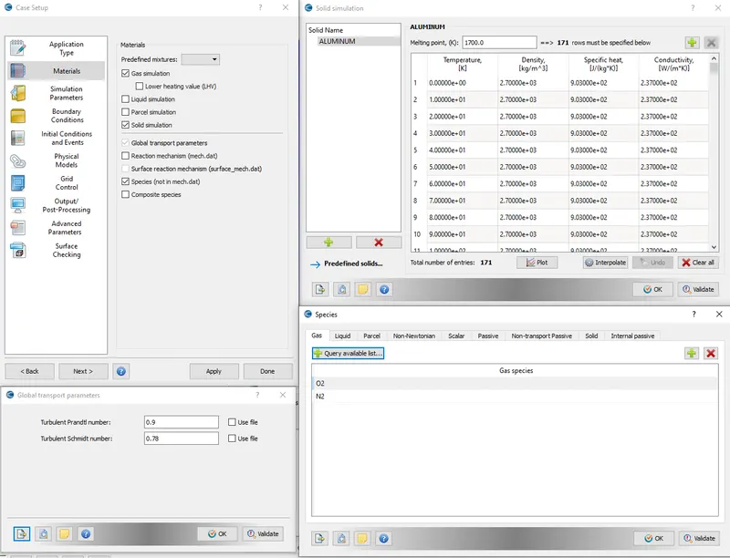
Air is chosen as the working fluid with 77% N2 and 23% O2. Aluminum is selected as the pipe material.

- Simulation Parameters:

The transient solver option is selected and respective settings for the conservation equations are defined:

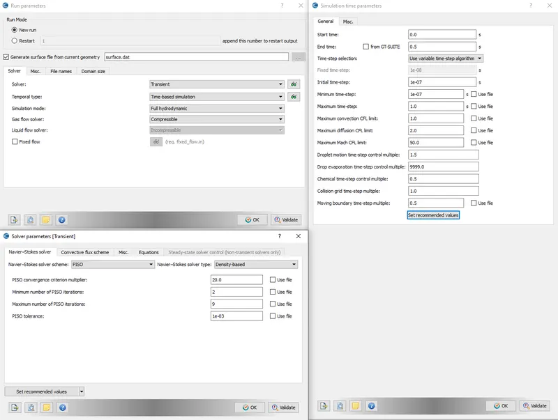
- Boundary Conditions:

The boundary conditions are assigned to the respective boundary zones in this menu. The applied boundary conditions are as follows:

Boundary Zone	Boundary condition
Solid outer wall	Type: Wall Velocity BC: - Stationary, Slip - Temperature BC: Heat flux = -10000 W/m^2 (heat flowing into the pipe)
Interface	Type: Interface (allows heat transfer interactions between solid pipe and flowing fluid) Boundary motion, Velocity BC: - Stationary - Forward side: Region: Fluid Velocity BC: Law of wall Temperature BC: Law of wall coupled - Reverse side: Region: Solid Wall treatment: Slip Temperature BC: Coupled
Solid side wall	Wall - Stationary, Slip, zero normal gradient temperature.
Inlet	Inflow: -Velocity BC: 3.572 m/s along Z-direction (this velocity coresponds to Re = 7000). -Temperature BC= 300 K - Species - O2 = 0.23, N2 - 0.77
Outlet	Outflow: -Pressure BC: 101325 Pa -Velocity BC: Zero normal gradient (NE) -Temperature BC: 300 K - Species Backflow: Mass Fraction Sum =1 (O2 0.23, N2 - 0.77)

The above boundary conditions can be defined only after defining a region in the Initial conditions and Events section of the case setup as shown below:

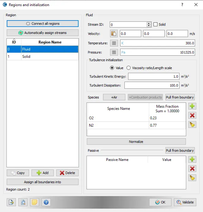
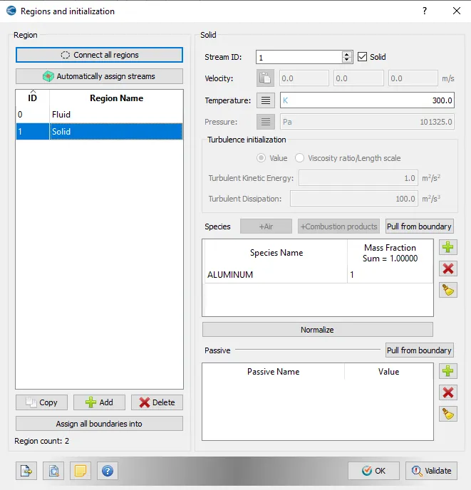
Two regions are created; one for fluid and the other for the solid pipe. The respective materials and stream ID are defined as shown in the above images.

Physical models:

Turbulence modeling:

Since the inlet flow is of Re= 7000, the flow is turbulent (for internal flows Re>2300). Hence the turbulence in the flow is modeled using RNG-K-ε">ε RANS model with standard wall function as shown below:

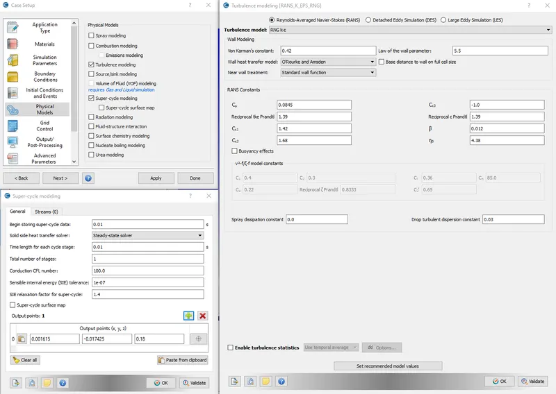
Also, the super cycling option is turned on with the respective settings as above. Super cycling is a method of solving the heat conduction equation in the solid region when a fluid-solid CHT is taking place. The solids usually possess a high value of specific heat when compared to fluids. The heat transfer in fluids reaches an equilibrium state faster than solids. To have equilibrium achieved in solids, super cycling enables after every time step completion, the fluid side analysis is halted until the solid side also reaches equilibrium before proceeding to the next time step. We can define monitor points to monitor the super cycling during the course of the simulation.

Grid control:

The mesh size for the domain is defined in this tab as shown below:

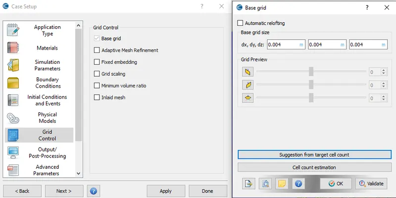
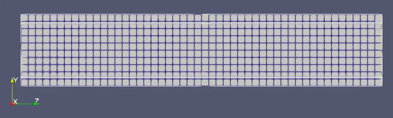
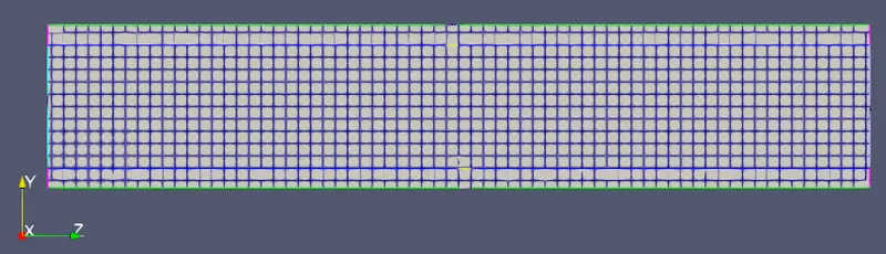
Three mesh sizes are considered for grid independence study in this analysis as below:

• Mesh1 - dx = dy = dz =4e-3 m
• Mesh2 - dx = dy = dz =3e-3 m
• Mesh3 - dx = dy = dz =2e-3 m

Output and post-processing:

The flow variables of interest, which are to be post-processed after the solution are selected in this option, and also at how many intervals these are written to the output file. Y-plus option is also selected in turbulence variables selection as shown below:

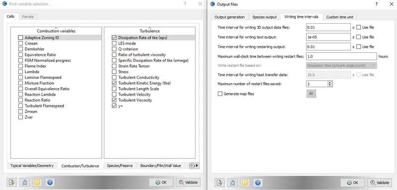
After all the above setup is completed final validation option is selected to check for the case setup is free of setup errors. After validation, the case setup files are exported using the export option in the File menu to the working folder. These files will be used by the CGYWIN terminal to run the solution. The above process is repeated for all the mesh sizes and the respective setup files are exported.

Solution in CYGWIN :

The solution is run in the CYGWIN terminal. First, we have to navigate to the respective working folder in the CYGWIN terminal, where case setup files are present. Then by executing the following command, the solution can be run:

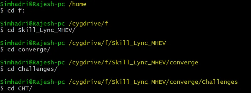
Executing the converge.exe using 4 parallel processors to run the solution:

The solution will run up to the simulation time set in the run setup and the output files are saved to the respective folders.

V Post-Processing Results:

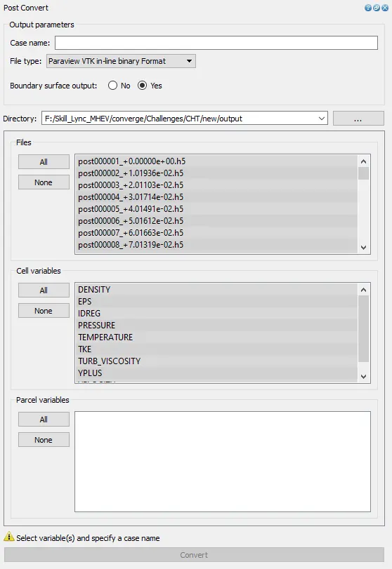
After the solution is complete, post-processing of the results is done using CONVERGE CFD and ParaView.

The plots are plotted in CONVERGE CFD, whereas to visualize the flow variables using contour plots the output files need to be converted to ParaView compatible files. This can be done in the CONVERGE CFD Post-Processing 3D tab as shown below:

Visualization in ParaView:

The converted ParaView compatible output files are opened in ParaView and the grid, contour plots for Pressure, Velocity, and velocity streamlines are visualized:

1. Grid 1 (dx = 4e-3m, dy = 4e-3m, dz = 4e-3m):

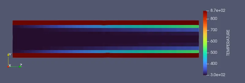
Temperature at the end of simulation:

2. Grid 2 (dx = 3e-3m, dy = 3e-3m, dz = 3e-3m):

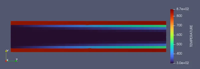
Temperature at the end of simulation:

3. Grid 3 (dx = 2e-3m, dy = 2e-3m, dz = 2e-3m):

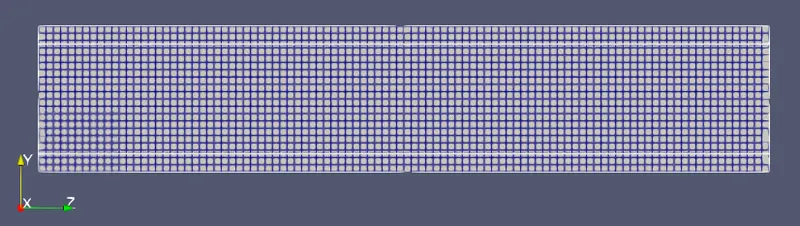
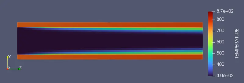
Temperature at the end of simulation:

Graph plots in Converge CFD:

The graphs are plotted for various flow variables using the line plotting tab in Converge CFD:

1. Grid 1 (dx = 4e-3m, dy = 4e-3m, dz = 4e-3m):

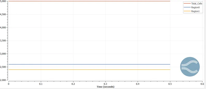
Total Cell count:

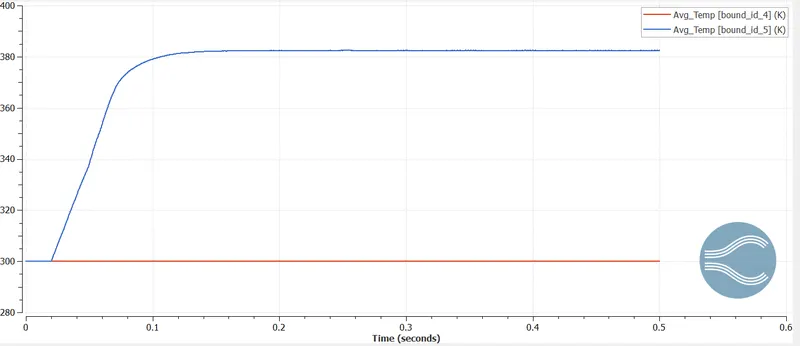
Temperature variation at the outlet over the course of simulation:

2. Grid 2 (dx = 3e-3m, dy = 3e-3m, dz = 3e-3m):

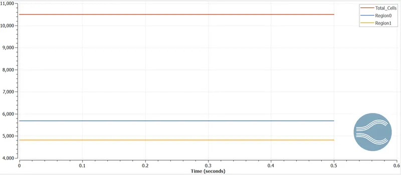
Total Cell count:

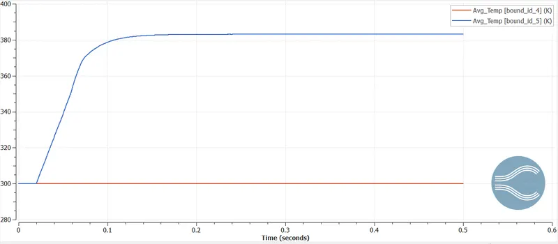
Temperature variation at the outlet over the course of simulation:

3. Grid 3 (dx = 2e-3m, dy = 2e-3m, dz = 2e-3m):

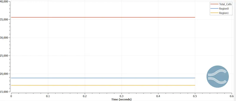
Total Cell count:

Temperature variation at the outlet over the course of simulation:

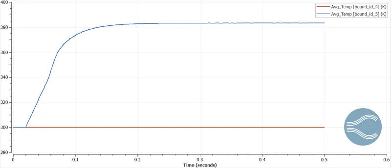
It can be seen from the above contour plots and graphs that the average outlet temperature reaches a steady-state value at around 315 K for all three grid sizes. But the temperature distribution reached uniformity at a cell size of 0.002 m. But the cell count increased to around 36000 when compared to 10500 (grid size of 0.003m). Considering the computational time and results quality grid size of 0.003 m is sufficient. Hence the analysis is grid-independent for a cell size of 0.003m.

The following animation shows the temperature variation in the solid region and fluid region over the course of simulation for the cell size of 0.02 m

It can be seen thermal boundary layer develops with an increase in thickness from the inlet of the pipe to the outlet.

Further, the supercycle stage interval is increased from baseline 0.01 s to 0.02 and 0.03 to see its effect on total simulation time for the cell size of 0.004 m case. The observations are as below:

Sl. No	Super cycle stage interval	Total Simulation time
1	0.01	720 sec
2	0.02	780 sec
3	0.03	900 sec

Conclusion:

In this project CHT simulation of heating a fluid flowing in a pipe is studied using transient analysis with the super-cycling method. The effect of grid size on the temperature distribution in the fluid is studied. Further, the effect of the super cycling stage interval is also studied for three different super cycling stage intervals.