Week 6: Conjugate Heat Transfer Simulation
Conjugate Heat Transfer Simulation
AIM: To perform Conjugate Heat Transfer flow simulation through a pipe using Converge CFD and post process the results using Paraview.
OBJECTIVE:
Setup a flow simulation through a pipe
Inner diameter 0.02mm
Outer diameter 0.015mm.
Inlet Reynolds number should be 7,000
Use the below formula to calculate velocity for Corresponding value of REYNOLD NUMBER and give DIRICHLET BC for velocity at inlet and specify the value for velocity calculated at INLET BC using below formula,
Re (rho*V*D)/(Dynamic viscosity)
Turbulence modelling - K-Epsilon
Supercycling parameters - same as in the video.
Additional 3D outputs
Add Y+ to your post.in file
Grid dependence test
Start with an initial base grid
Run grid dependence test on 3 grids and show that the outlet temperature converges to a particular value
Effect of supercycle stage interval.
Set supercyle stage interval to 0.01,0.02 and 0.03.
For these three values, how does the total simulation time compare against the baseline configuration.
Introduction:
When multiple modes of heat transfer ie., variations of temperature within solids and fluids, due to thermal interaction between the solids and fluids are involved then the process is called Conjugate Heat Transfer.
Wall functions are useful in calculation the solutions near the wall. Y+ is a dimensionaless quantity that can be used to understand whether the mesh is coarse or fine which in turn determines the need for wall functions. The Turbulent flow have a smaller laminar region near the wall and if we are to resolve the gradients at such a small region, very small grid size is required.
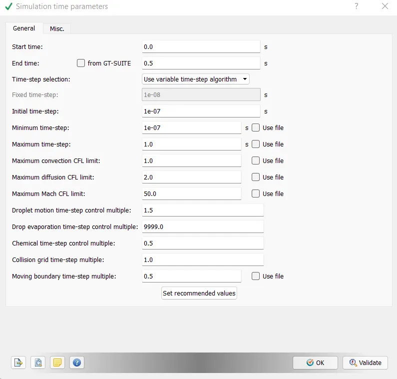
Super cycling is a method that is used to solve CHT simulations in converge. In this method solver solves the solid region and fluid region seperately. The time scale difference between both the fluid and solid regions is very high as the time required for solver to attain steady state in fluid region is very small when compared to that of solid. In supercycling, the solver of the fluid domain is paused untill the solid domain reaches steady state. This pausing is called as supercycling stage interval and it is user defined in pre processing.
Initially, for 0.1s, both the fluid domain and solid domain solvers are run. At first interval, 0.1s, the fluid solver is paused and the solid side solver is continued to run towards convergence.
STEPS:
- CHT Modeling Setup
- There are several steps to setting up a CHT simulation
- Define fluid and solid materials and their physical properties
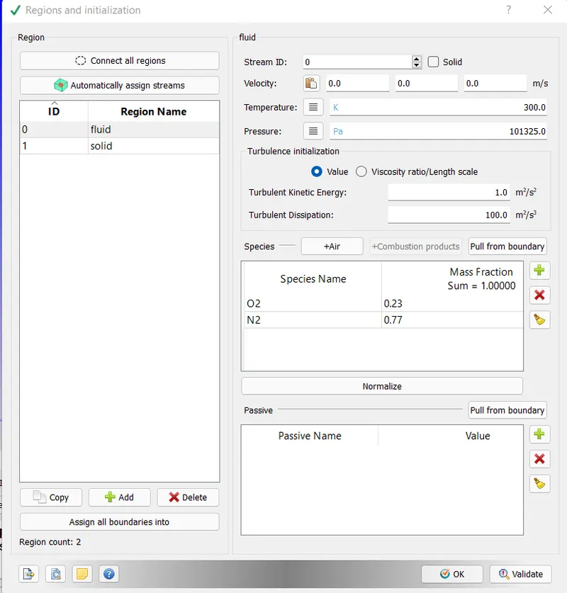
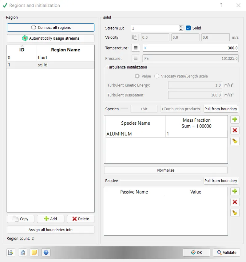
- Configure the fluid and solid regions
- Assign regions to streams
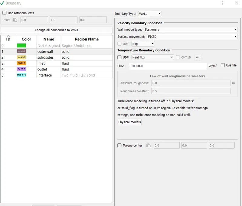
- Use appropriate boundary conditions for the boundaries that separate different regions
- Select time control method (transient, steady-state, or super-cycle)
- Set up post-processing
Geometry setup
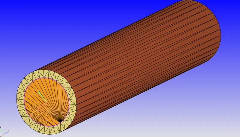
Time base case setup
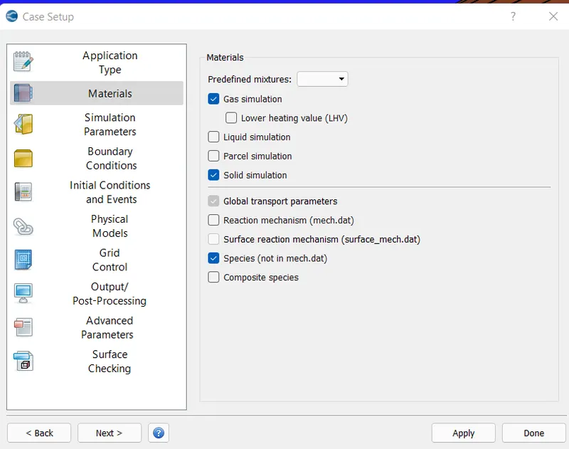
Select gas ,solid , simulation
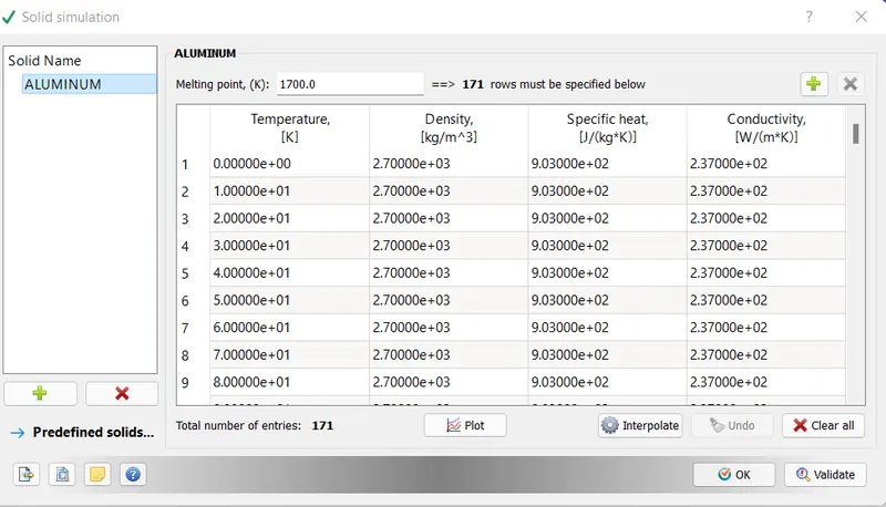
Select Alimunum as a solid species
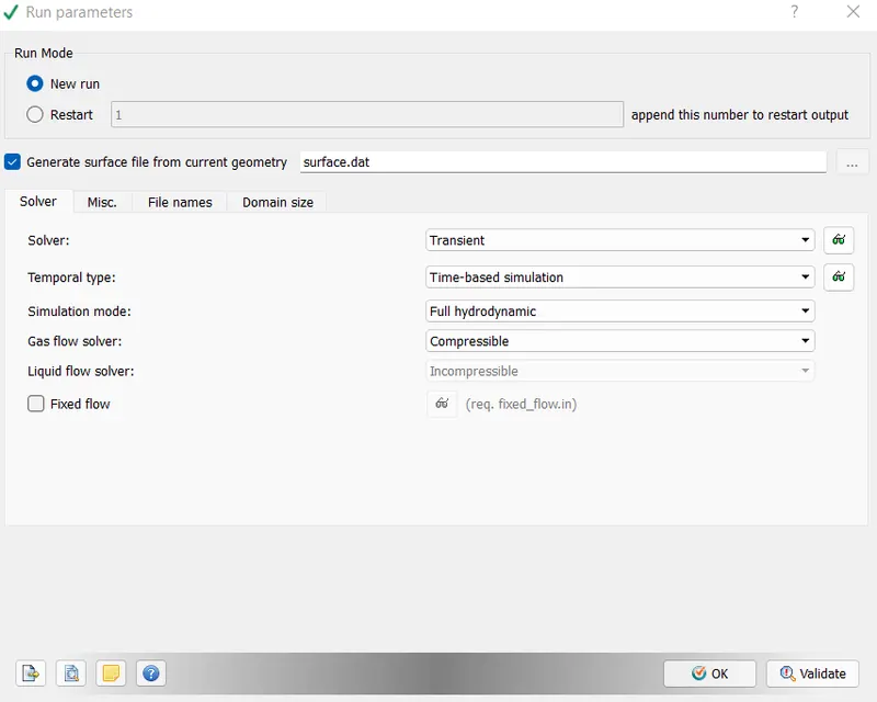
Trasient solver
Inlet:
Neumann boundary condition for pressure
Dirchelet boundary condition for velocity. This is calculated usind reynols number=7000
Re= p. V. D μ
Re = 7000
Density of air = 1.225 kg/m^3
Viscosity = 1.81e-5 kg.m/s
Hence, Velocity = 2.78m/s
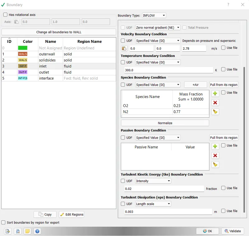
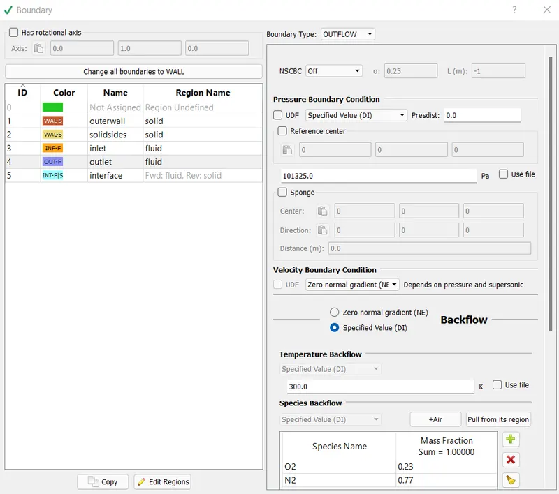
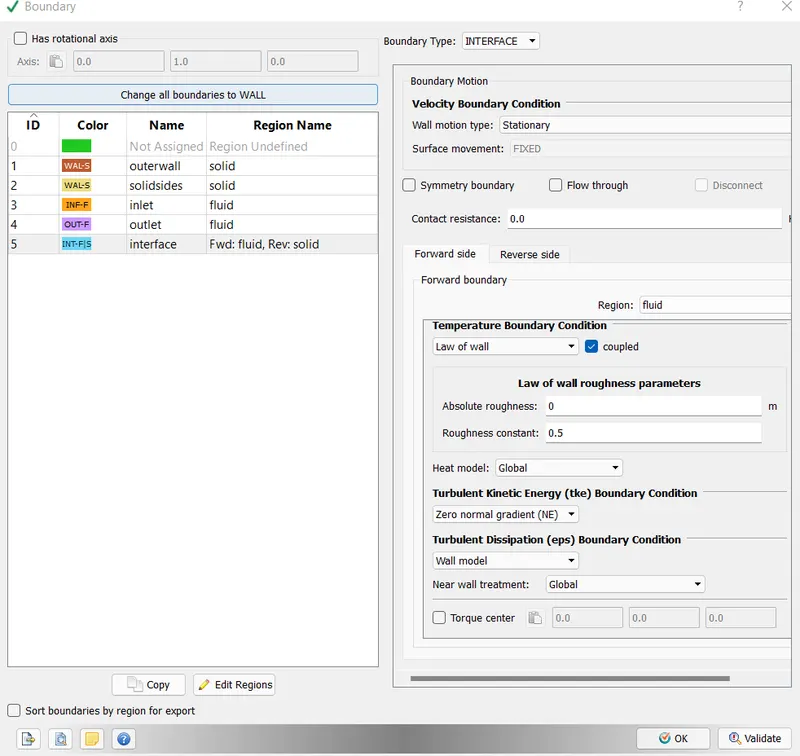
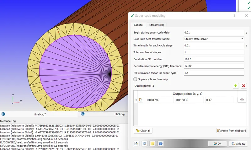
paste the location in the output files
at the Z direction input 0.17 because we can see the simulation near the end
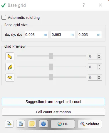
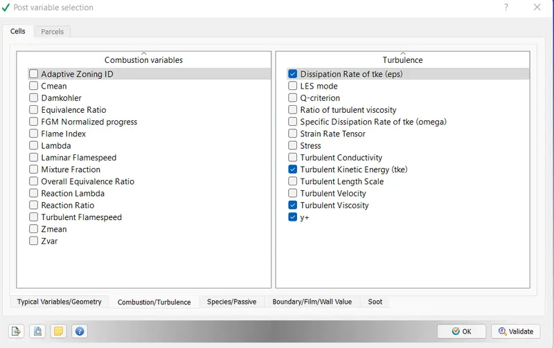
Check the Y+ for the results
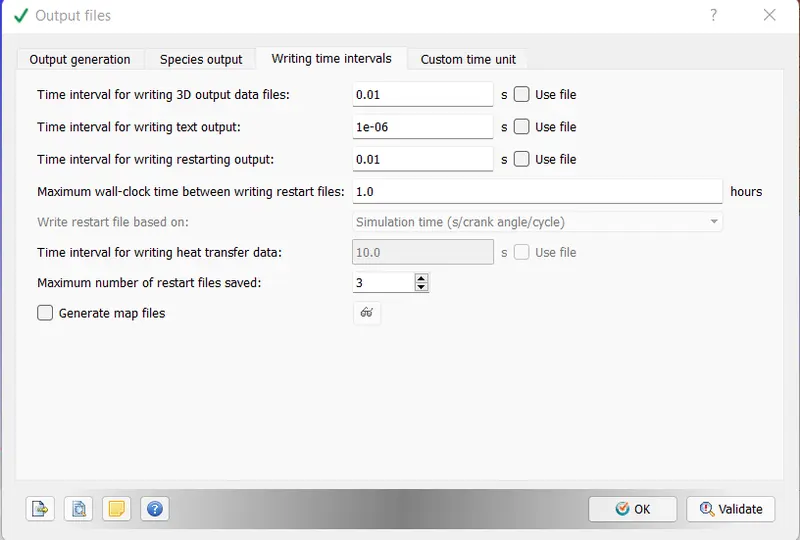
Save the outputs files and run through CIGWIN commands
And postProcess the files and Open in paraview and check the grids and animation of the Temprature and Y+
Effect of Super Cycle Stage interval
Case 1: Gride size=0.005 and supercyle stage interval=0.01
Case 2: Gride size=0.003 and supercyle stage interval=0.02
Case 3: Gride size=0.003 and supercyle stage interval=0.03
Hear are the polts and the images for the CHT
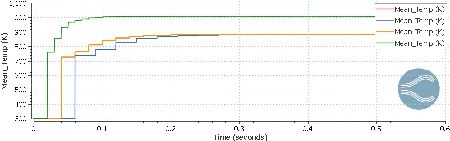
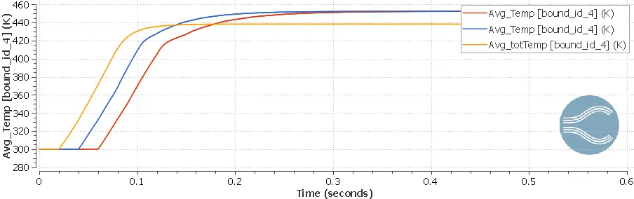
We can see here that the temperature is dependant on the grid size. More the temperature more will be the grid spacing and viceversa
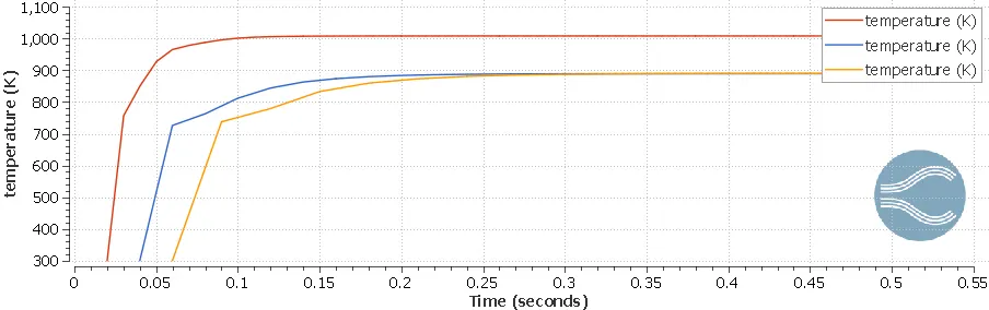
SUPER CYCLING VS SIMULATION TIME:
We are having a base grid of 4mm as a baseline configuration and then we are decreasing the interval for supercycling from 0.03.0.02.
0.01.
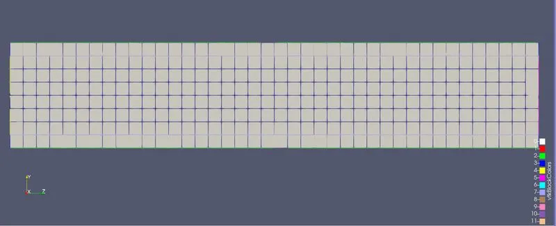
0.05baseGrid 0.01 supercyle stage interval
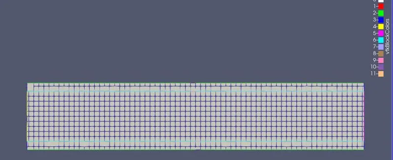
0.03baseGrid(0.02)supercycle
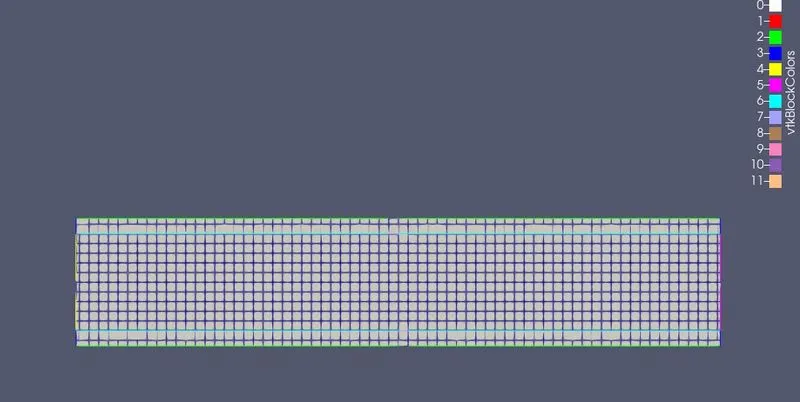
0.03grid(0.03)supercycle
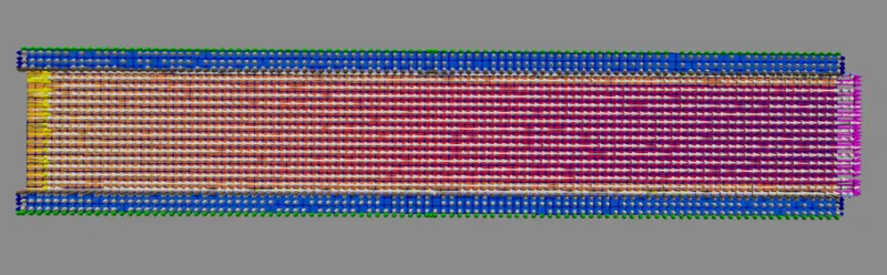
Vector plot
YouTube links for the animations
CONCLUSION:
It is clear from the Mean Temp Vs Time Plot of fluid and solid that the time scale difference between both the fluid and solid regions is very high as the time required for soliver to attain steady state in fluid region is very small when compared to that of solid
Supercycling interval decreases the simulation time increases
The study of Conjugate Heat Tranfer through a pipe using Converge CFD and Paraview was simulated successfully