Week 7 - Simulation of a 1D Super-sonic nozzle flow simulation using Macormack Method
OBJECTIVE
To simulate the isentropic flow through a crazy wonder subsonic and supersonic nozzle using both conservation and on conservation forms of governing equation and solve them using the Micromax technique and compare their solution
We consider the study fashion traffic flow through a convergent divergent nozzle the flow at the inlet to the nozzle comes from the reservoir the cross section area of the reservoir is very large and hence velocity is very small the flow is locally subsonic the convergent section of the nozzle sonic and a supersonic at divergent section.
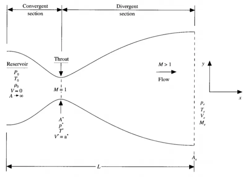
Consider a small control vloume of a nozzle and apply the conservation equation to them
We should solve to problem by using the MacCormack's technique.
the step involve
- Initial profile
- preditor step
- solution update
- correcter step
- Final soluction
MAIN CODE
clear all
close all
clc
L = 3;
n = [31];
cfl = 0.5;
nt=1:1400;
for i = 1:length(n)
x = linspace(0,L,n(i));
[mfr_c,mfr_throat_c] = conservative(L,n(i),nt,cfl)
[mfr_nc,mfr_throat_nc] = non_conservative(L,n(i),nt,cfl)
figure(7)
plot(nt,mfr_nc,'b',nt,mfr_c,'r','linewidth',1)
xlabel('time step (nt)')
ylabel('mass flow rate')
legend('conservative form','Non conservation form')
title('mass flow rate using "Non conservationform vs conservationform" at throat point i=16')
figure(8)
plot(nt,mfr_throat_c,'b',nt,mfr_throat_nc,'r','linewidth',1)
xlabel('time step (nt)')
ylabel('mass flow rate')
legend('conservative form','Non conservation form')
title('mass flow rate using "Non conservationform vs conservationform" at trooat point i=16')
end
******* Conservation CODE***********
function [mfr_c,mfr_throat_c] = conservative(L,n,nt,cfl)
x = linspace(0,L,n);
dx = x(2)-x(1);
cfl=0.5;
%initial condition rho,a,v,T,M,mfr,p
for ii=1:length(x)
if (x(ii)<=0.5)
rho(ii)=1;
T(ii)=1;
elseif(x(ii)>0.5) & (x(ii)<=1.5)
rho(ii) = 1-0.366*(x(ii)-0.5);
T(ii)=1-0.167*(x(ii)-0.5);
elseif(x(ii)>1.5)&(x(ii)<=3.5);
rho(ii) = 0.634-0.3879*(x(ii)-1.5);
T(ii)=0.833-0.3570*(x(ii)-1.5);
end
end
a=1+2.2*(x-1.5).^2;
g=1.4;
%soluction vector
u1=rho.*a;
u2=0.59*ones(1,n);
v=u2./u1;
u3=u1.*((T./(g-1))+(g/2).*v.^2);
M=v./(T.^0.5);
mfr=rho.*a.*v;
p=rho.*T;
for z=1:31 %find dt
u=(T(z))^(1/2);
dt(z)= cfl*dx/(u+v(z));
end
dt=min(dt);
for i = 1:length(nt)
%sorting initiak value
u1_old=u1;
u2_old=u2;
u3_old=u3;
for j=2:n-1
%flux vector
f1=u2
f2=((u2.^2)./u1)+((g-1)/g)*(u3-((g/2)*(u2.^2)./u1));
f3=((g.*u2.*u3)./u1)-((g*(g-1)/2)*(u2.^3)./(u1.^2));
%sourece terminal_size
j1=(1/g)*rho(j)*T(j)*((a(j+1)-a(j))/dx);
%predector step
du1dt_p(j)=-(f1(j+1)-f1(j))/dx;
du2dt_p(j)=-(f2(j+1)-f2(j))/dx+j1;
du3dt_p(j)=-(f3(j+1)-f3(j))/dx;
%updating soluction
u1(j)=u1_old(j)+du1dt_p(j)*dt;
u2(j)=u2_old(j)+du2dt_p(j)*dt;
u3(j)=u3_old(j)+du3dt_p(j)*dt;
%updating primitive
rho=u1./a;
T=(g-1).*(u3./u1-(g/2).*(u2./u1).^2);
%updating flux
f1=u2;
f2=u2.^2./u1+((g-1)/g).*(u3-(g/2)*u2.^2./u1);
f3=g.*u2.*u3./u1-0.5*g*(g-1).*u2.^3./u1.^2;
%source term for coorector step
j2=(1/g)*(rho(j)*T(j)*(a(j)-a(j-1))/dx);
%corrector step
du1dt_c(j)=-(f1(j)-f1(j-1))/dx;
du2dt_c(j)=-(f2(j)-f2(j-1))/dx+j2;
du3dt_c(j)=-(f3(j)-f3(j-1))/dx;
end
%average time deritive
du1dt_avg=0.5*(du1dt_p+du1dt_c);
du2dt_avg=0.5*(du2dt_p+du2dt_c);
du3dt_avg=0.5*(du3dt_p+du3dt_c);
%final correctors value
for k=2:n-1;
u1(k)=u1_old(k)+du1dt_avg(k)*dt;
u2(k)=u2_old(k)+du2dt_avg(k)*dt;
u3(k)=u3_old(k)+du3dt_avg(k)*dt;
end
%entry boundary
u1(1)=a(1);
u2(1)=2*u2(2)-u2(3);
u3(1)=u1(1)*(T(1)/(g-1)+(g*(u2(1)/u1(1))^2)/2);
%exit boundry condition
u1(n)=2*u1(n-1)-u1(n-2);
u2(n)=2*u2(n-1)-u2(n-2);
u3(n)=2*u3(n-1)-u3(n-2);
%final update primitive
rho=u1./a;
v=u2./u1;
T=(g-1).*(u3./u1-(g/2).*(u2./u1).^2);
p=rho.*T;
M=v./T.^0.5;
error(k)= abs(v(k)-v(k-1));
mfr=u2;
%to find the value of throat point
T_throat(i)=T(16);
rho_throat(i)=rho(16);
v_throat(i)=v(16);
M_throat(i)=M(16);
p_throat(i)=p(16);
error_throat(i)=error(16);
mfr_throat(i)=mfr(16);
if n==31
for ii=[1:50:201 700]
if ii==i
figure(4)
plot(x,mfr,'linewidth',1)
hold on
title('conservative form -varation of mfr inside the nozzle at differnt time step')
xlabel('length of nozzle')
ylabel('mass flow rate')
elseif i==1400
plot(x,mfr,'*r')
legend('@1','@50','@150','@200','@700','@1400')
endif
endfor
endif
endfor
if n==31
figure(5)
plot(x,v,'b',x,p,'r',x,T,'k',x,rho,'m',x,M,'g',x,mfr,'c')
ylim([-0.1 3.7])
title(sprintf('time step =%d',i))
xlabel('length of nozzle')
ylabel('Non dimensional parameters')
legend('velocity','presure','Temprature','density','Mass floe rate','Mach number','location','northwest')
title('conservative form - steady state primitives variables inside the nozzle')
figure(6)
plot(nt,rho_throat)
hold on
plot(nt,v_throat,'linewidth',1)
plot(nt,p_throat,'linewidth',1)
plot(nt,T_throat,'linewidth',1)
plot(nt,M_throat,'linewidth',1)
plot(nt,mfr_throat,'linewidth',1)
xlabel('time step')
ylabel('Non dimensional parameters')
legend('velocity','presure','Temprature','density','Mass floe rate','Mach number')
title('conservative form - Time wise variation of primitive variable at throat poini i=16')
endif
mfr_c=mfr;
mfr_throat_c=mfr_throat;
end
******************NON Conservation*************
function [mfr_nc,mfr_throat_nc] = non_conservative(L,n,nt,cfl)
x = linspace(0,L,n);
dx = x(2)-x(1);
%initial condition rho,a,v,t,mfr,M,p
rho = 1-0.3146*x;
T = 1-0.2314*x;
v = (0.1+1.09*x).*T.^0.5;
a = 1+2.2*(x-1.5).^2;
M = v./(T.^0.5);
mfr = rho.*a.*v;
p = rho.*T;
cf1=0.5;
g = 1.4;
for z = 1:31
u = (T(z))^(1/2);
dt(z) = cf1*dx/(u+v(z));
end
dt = min(dt);
for i = 1:nt
%sorting initial value
rho_old = rho;
told = T;
vold = v;
for j = 2:n-1
%predictor step
drhodx = (rho(j+1)-rho(j))/dx;
dvdx = (v(j+1)-v(j))/dx;
dtdx = (T(j+1)-T(j))/dx;
dlogadx = (log(a(j+1))-log(a(j)))/dx;
drhodt_p(j) = -rho(j)*dvdx-rho(j)*v(j)*dlogadx-v(j)*drhodx;
dvdt_p(j) = -v(j)*dvdx-(1/g)*(dtdx+(T(j)/rho(j)))*drhodx;
dtdt_p(j) = -v(j)*dtdx-(g-1)*T(j)*(dvdx+v(j)*dlogadx);
%updating primiritves
v(j) = v(j)+dvdt_p(j)*dt;
rho(j) = rho(j)+drhodt_p(j)*dt;
T(j) = T(j)+dtdt_p(j)*dt;
%corrector step
drhodx = (rho(j)-rho(j-1))/dx;
dvdx = (v(j)-v(j-1))/dx;
dtdx = (T(j)-T(j-1))/dx;
dlogadx = (log(a(j))-log(a(j-1)))/dx;
drhodt_c(j) = -rho(j)*dvdx-rho(j)*v(j)*dlogadx-v(j)*drhodx;
dvdt_c(j) = -v(j)*dvdx-(1/g)*(dtdx+(T(j)/rho(j))*drhodx);
dtdt_c(j) = -v(j)*dtdx - (g-1)*T(j)*(dvdx+v(j)*dlogadx);
end
%average time dreative
drhodt_avg = 0.5*(drhodt_p+drhodt_c);
dvdt__avg = 0.5*(dvdt_p+dvdt_c);
dtdt_avg = 0.5*(dtdt_p+dtdt_c);
%final correct value
for k = 2:n-1
rho(k) = rho_old(k)+drhodt_avg(k)*dt;
v(k) = vold(k)+dvdt__avg(k)*dt;
T(k) = told(k)+dtdt_avg(k)*dt;
end
%entry boundry condition
v(1) = 2*v(2)-v(3);
%exit boundry condition
v(n) = 2*v(n-1)-v(n-2);
rho(n) = 2*rho(n-1)-rho(n-2);
T(n) = 2*T(n-1)-T(n-2);
%final update for primitives
p = rho.*T;
M = v./T.^0.5;
error(k) = abs(v(k)-v(k-1));
mfr = rho.*a.*v;
%to find the value of throat point
T_throat(i) = T(16);
rho_throat(i) = rho(16);
v_throat(i) = v(16);
M_throat(i) = M(16);
p_throat(i) = p(16);
error_throat(i) = error(16);
mfr_throat(i) = mfr(16);
figure(3) non conservative
plot(rho_throat,'linewidth',1)
hold on
plot(v_throat,'linewidth',1)
plot(p_throat,'linewidth',1)
plot(T_throat,'linewidth',1)
plot(M_throat,'linewidth',1)
plot(mfr_throat,'linewidth',1)
xlabel('time step')
ylabel('non dimesion parameter')
legend('density','velocity','pressure','temprature','Mach number','Mass flow rate ')
title('Non conservative form - time wise varation of varabiles at point i-16')
if n==31
for ii=[1:50:201 700]
if ii=i
figure(1)
plot(x,mfr,'linewidth',1)
hold on
title('Non conservative form-varation of mas fkow rate inside the nozzle at the differenr time marching')
xlabel('length of nozzle')
ylabel('mass flow rate')
elseif i==1400
plot(x,mfr,'*r')
legend('@1','@50','@101','@152','@201','@700','@1400')
endif
end
end
end
if n==31
figure(2)
plot(x,v,'b')
hold on
plot(x,p,'r')
plot(x,T,'k')
plot(x,rho,'m')
plot(x,M,'g')
ylim([-0.1 3.7])
title(sprintf('timestep = %d',i));
xlabel('length of nozzle')
ylabel('non dimesion parameter')
legend('Velocity','Pressure','Temperature','Density')
title('Non conservative form - stedy state distrubtion of variables inside nozzle')
end
mfr_nc=mfr;
mfr_throat_nc=mfr_throat;
end
Figure 1 shows study study distribution of non dimensional primitive variables at the end of a timestamp this value of of flow field variable applying the exact value shown in the John d Anderson book
The figure 2 shows time wise variation of a primitive variable at third point is equal to 16 around the time step of 500 the flow field variable obtained stable solution
In the figure 3 e shows the variation of mass flow rate distribution inside the nozzle at different times during the time marking process the mass floor and finally settled at 0.58
Figure 4 shows study state distribution of non dimensional primitive variable at the end of a timestamp value of the flow field variable applies as the exact value shown in the book
Figure 5 shows a variation of a primitive variable atta 3.16 around the time step of 600D flow field variable obtained in a stable solution
The figure 6 shows the variation of mass flow rate distribution inside the nozzle at different time steps during the time marketing process the mass flow rate finally settled at 0.5
The figure Airtel 9 shows the comparison and moment of mass flow rate with the respective X
The initial and boundry condition are referef as in the john D andreson textBook.