Week 3.5 - Deriving 4th order approximation of a 2nd order derivative using Taylor Table method

AIM:

4th order approximations of the second-order derivative.

1. Central difference

2. Skewed right-sided difference

3. Skewed left-sided difference

Skewed right hand difference scheam

Number of nodes N=P+Q P=oredr of derivative

Q=order of approximation

N=2+4=6

To derive the fourth order approximatiom for the second order derivative .

We start with the approximation

Expand All the terms in the equation forms using the tylor seriws expansion and are represents in the form of a table

d^2/dx^2	f(i)	Δxf'(i)	Δx^2f(i)	Δx^3f(i)	Δx^4f(i)	Δx^5f(i)
af(i)	a	0	0	0	0	0
bf(i+1)	b	b	b/2	b/6	b/24	b/120
cf(i+2)	c	2c	4c/2	8c/2	16c/2	32c/2
df(i+3)	d	3d	9d/2	27d/6	81d/24	243d/120
ef(i+4)	e	4e	16e/2	64e/6	256e/24	1024e/120
gf(i+5)	g	5g	25g/2	125g/6	625g/24	3125g/120
sum of co efficent	0	0	1	0	0	0

The linear equation are in the above equation solve this using matrix inversion method

A.X=B

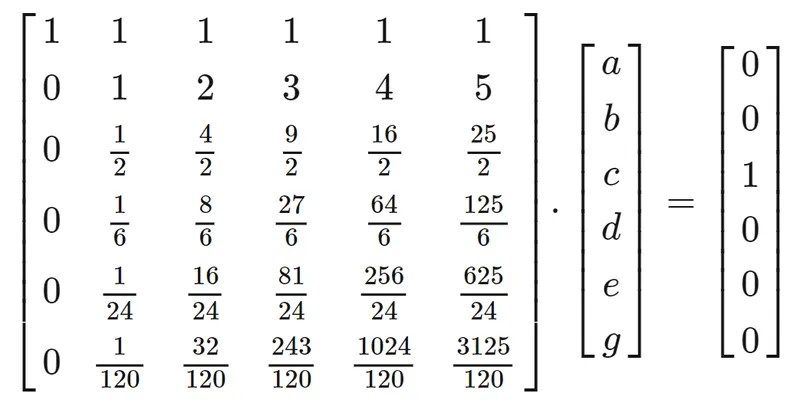
A=[1 1 1 1 1 1;0 1 2 3 4 5;0 1/2 4/2 9/2 16/2 25/2;0 1/6 8/6 27/6 64/6 125/6;0 1/24 16/24 81/24 256/24 625/24;0 1/120 32/120 243/120 1024/120 3125/120]
B=[0;0;1;0;0;0]

X=inv(A)*B

A =

1.0000 1.0000 1.0000 1.0000 1.0000 1.0000
0 1.0000 2.0000 3.0000 4.0000 5.0000
0 0.5000 2.0000 4.5000 8.0000 12.5000
0 0.1667 1.3333 4.5000 10.6667 20.8333
0 0.0417 0.6667 3.3750 10.6667 26.0417
0 0.0083 0.2667 2.0250 8.5333 26.0417

B =

0
0
1
0
0
0

X =

3.7500
-12.8333
17.8333
-13.0000
5.0833
-0.8333

Skewed left hand difference scheam

Number of nodes N=P+Q P=oredr of derivative

Q=order of approximation

N=2+4=6

To derive the fourth order approximatiom for the second order derivative .

We start with the approximation

Expand All the terms in the equation forms using the tylor series expansion and are represents in the form of a table

d^2/dx^2	f(i)	Δxf'(i)	Δx^2f(i)	Δx^3f(i)	Δx^4f(i)	Δx^5f(i)
af(i-5)	a	-5a	25a/2	-125a/6	625a/24	3125a/120
bf(i-4)	b	-4b	16b/2	-64b/6	256b/24	b/120
cf(i-3)	c	-3c	9c/2	-27c/6	-27c/6	32c/2
df(i-2)	d	2d	4d/2	-8d/6	-8d/6	243d/120
ef(i-1)	e	-e	e/2	-e/2	-e/6	1024e/120
gf(i)	g	0	0	0	0	0
sum of co efficent	0	0	1	0	0	0

The linear equation are in the above equation solve this using matrix inversion method

A.X=B

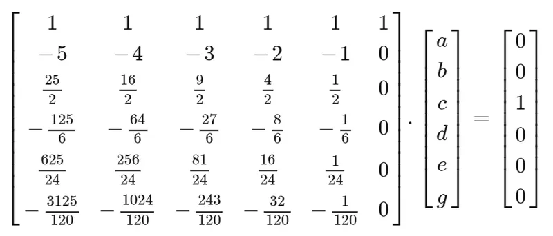
A=[1 1 1 1 1 1;-5 -4 -3 -2 -1 0;25/2 16/2 9/2 4/2 1/2 0;-125/6 -64/6 -27/6 -8/6 -1/6 0;625/24 256/24 81/24 16/24 1/24 0;-3125/120 -1024/120 -243/120 -32/120 -1/120 0]
B=[0;0;1;0;0;0]

X=inv(A)*B

A =

1.0000 1.0000 1.0000 1.0000 1.0000 1.0000
-5.0000 -4.0000 -3.0000 -2.0000 -1.0000 0
12.5000 8.0000 4.5000 2.0000 0.5000 0
-20.8333 -10.6667 -4.5000 -1.3333 -0.1667 0
26.0417 10.6667 3.3750 0.6667 0.0417 0
-26.0417 -8.5333 -2.0250 -0.2667 -0.0083 0

B =

0
0
1
0
0
0

X =

-0.8333
5.0833
-13.0000
17.8333
-12.8333
3.7500

central difference scheam

A=[1 1 1 1 1 ;-2 -1 0 1 2 ;2 1/2 0 1/2 2;-4/3 -1/6 0 1/6 4/3;2/3 1/24 0 1/24 2/3]
B=[0;0;1;0;0]

X=inv(A)*B

A =

1.0000 1.0000 1.0000 1.0000 1.0000
-2.0000 -1.0000 0 1.0000 2.0000
2.0000 0.5000 0 0.5000 2.0000
-1.3333 -0.1667 0 0.1667 1.3333
0.6667 0.0417 0 0.0417 0.6667

B =

0
0
1
0
0

X =

-0.083333
1.333333
-2.500000
1.333333
-0.083333

Center difference scheam

Number of nodes N=P+Q-1 P=oredr of derivative

Q=order of approximation

N=2+6-1=5

To derive the fourth order approximatiom for the second order derivative .

We start with the approximation

Expand All the terms in the equation forms using the tylor series expansion and are represents in the form of a table

d^2/dx^2	f(i)	Δxf'(i)	Δx^2f(i)	Δx^3f(i)	Δx^4f(i)
af(i-2)	a	-2a	2a	-4a/3	-4a/3
bf(i-1)	b	4b	b/2	-b/6	-b/6
cf(i)	c	0	0	0	0
df(i+1)	d	d	ed/2	d/6	d/6
ef(i+2)	e	2e	2e	4e/3	4e/3
sum of co efficent	0	0	1	0	0

A.X=B

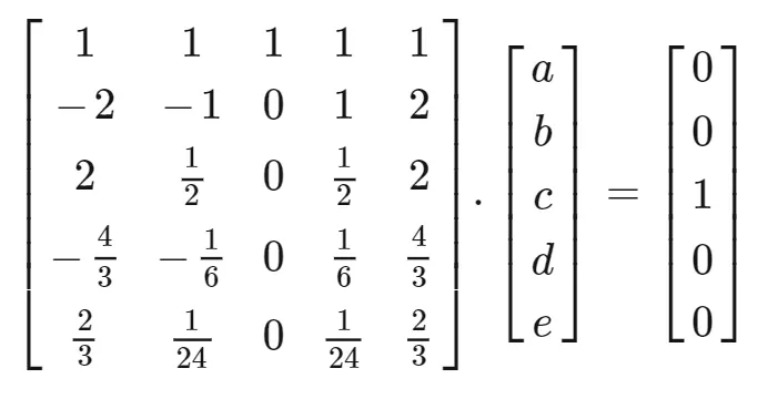
A=[1 1 1 1 1 ;-2 -1 0 1 2 ;2 1/2 0 1/2 2;-4/3 -1/6 0 1/6 4/3;2/3 1/24 0 1/24 2/3]
B=[0;0;1;0;0]

X=inv(A)*B

A =

1.0000 1.0000 1.0000 1.0000 1.0000
-2.0000 -1.0000 0 1.0000 2.0000
2.0000 0.5000 0 0.5000 2.0000
-1.3333 -0.1667 0 0.1667 1.3333
0.6667 0.0417 0 0.0417 0.6667

B =

0
0
1
0
0

X =

-0.083333
1.333333
-2.500000
1.333333
-0.083333

Main code

clear all
close all
clc

%inputs
x=pi/3;
analytical_derivative = -2*exp(x)*sin(x);

%central differecing
A=[1 1 1 1 1;-2 -1 0 1 2;2 1/2 0 1/2 2;-4/3 -1/6 0 1/6 4/3;2/3 1/24 0 1/24 2/3];
B=[0;0;1;0;0]
C=inv(A)*B;

% skewde left sided differencing

G=[1 1 1 1 1 1;-5 -4 -3 -2 -1 0;25/2 16/2 9/2 4/2 1/2 0;-125/6 -64/6 -27/6 -8/6 -1/6 0;625/24 256/24 81/24 16/24 1/24 0;-3125/120 -1024/120 -243/120 -32/120 -1/120 0];
H=[0;0;1;0;0;0];

I=inv(G)*H;

%skewde right sided differencing
D=[1 1 1 1 1 1;0 1 2 3 4 5;0 1/2 4/2 9/2 16/2 25/2;0 1/6 8/6 27/6 64/6 125/6;0 1/24 16/24 81/24 256/24 625/24;0 1/120 32/120 243/120 1024/120 3125/120];
E=[0;0;1;0;0;0];

F=inv(D)*E;

%numerical derivative
dx=linspace(pi/3,pi/200,20);

for i=1:length(dx)

central_differencing(i) = (C(1)*exp(x-2*dx(i))*cos(x-2*dx(i))+C(2)*exp(x-dx(i))*cos(x-dx(i))+C(3)*exp(x)*cos(x)+C(4)*exp(x+dx(i))*cos(x+dx(i))+C(5)*exp(x+2*dx(i))*cos(x+2*dx(i)))/dx(i)^2;

left_skewed_differencing(i) = (I(1)*exp(x)*cos(x)+I(2)*exp(x-5*dx(i))*cos(x-5*dx(i))+I(3)*exp(x-4*dx(i))*cos(x-4*dx(i))+I(4)*exp(x-3*dx(i))*cos(x-3*dx(i))+I(5)*exp(x-2*dx(i))*cos(x-2*dx(i))+I(6)*exp(x-1*dx(i))*cos(x-1*dx(i)))/dx(i)^2;

right_skewed_differencing(i) = (F(1)*exp(x)*cos(x)+F(2)*exp(x+dx(i))*cos(x+dx(i))+F(3)*exp(x+2*dx(i))*cos(x+2*dx(i))+F(4)*exp(x+3*dx(i))*cos(x+3*dx(i))+F(5)*exp(x+4*dx(i))*cos(x+4*dx(i))+F(6)*exp(x+5*dx(i))*cos(x+5*dx(i)))/dx(i)^2;

end

error_central = abs(central_differencing-analytical_derivative);
error_left = abs(left_skewed_differencing-analytical_derivative);
error_right = abs(right_skewed_differencing-analytical_derivative);

%polt

loglog(dx,error_central,'b',error_left,'r',error_right,'g');
hold on
xlabel('dx');
ylabel('error');
legend('central','left','right');
title('range of dx vs error')

Importance of skewed scheam

you can observe in thr graph we can compute from front,back and even middle of the equation,

The center scheam is having a less error compare to the other two and gives the value from the both sided for the equation.the system which do not contain enough information from the direction and which derivetive order we requried the answer at the time we can use the skewed differencing with the multiple value using the taylors series table