CHT Analysis on a Graphics card

AIM:

The aim of this project is to simulate conjugate heat transfer on a graphics card.

OBJECTIVES OF THE PROJECT:

1. Run the simulation by varying the velocity from 1m/sec to 5m/sec for at least 3 velocities.
2. Find the maximum temperature and heat transfer coefficient attained by the processor.
3. Check if the simulation has achieved convergence with appropriate images and plots.
4. Identify potential hotspots on the model.

THEORY:

What is Conjugate heat transfer?

Conjugate heat transfer corresponds with the combination of heat transfer in solids and heat transfer in fluids. In solids, conduction often dominates whereas, in fluids, convection usually dominates. Conjugate heat transfer is observed in many situations. For example, heat sinks are optimized to combine heat transfer by conduction in the heat sink with the convection in the surrounding fluid.

Where is CHT used?

CHT is used in designing heat exchangers, Energy Savings, Cooling of eletronic devices such as graphic cards, It can be used in places when there is a heat transfer between a solid and fluid.

In this project, we will setup conjugate heat transfer through an exhaust manifold and observe various parameters.

PROCEDURE:

Importing the geometry

For our case the geometry was already created. This is a model of a graphics card and it can be found here.

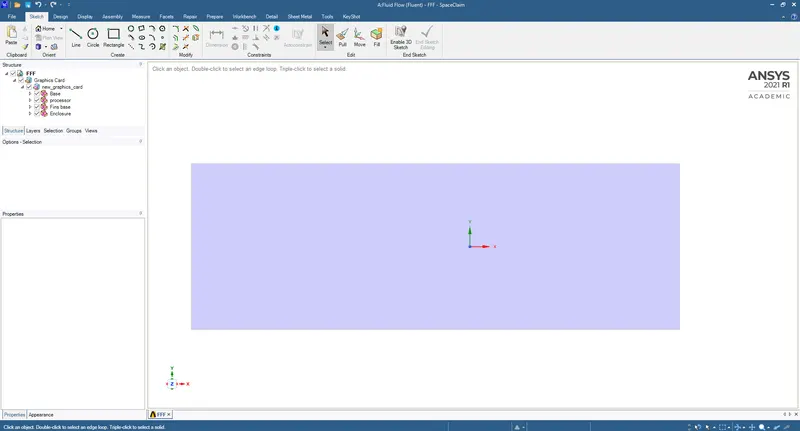
We start with importing this geometry into Ansys Fluent using the drag and drop option. The geometry is as shown

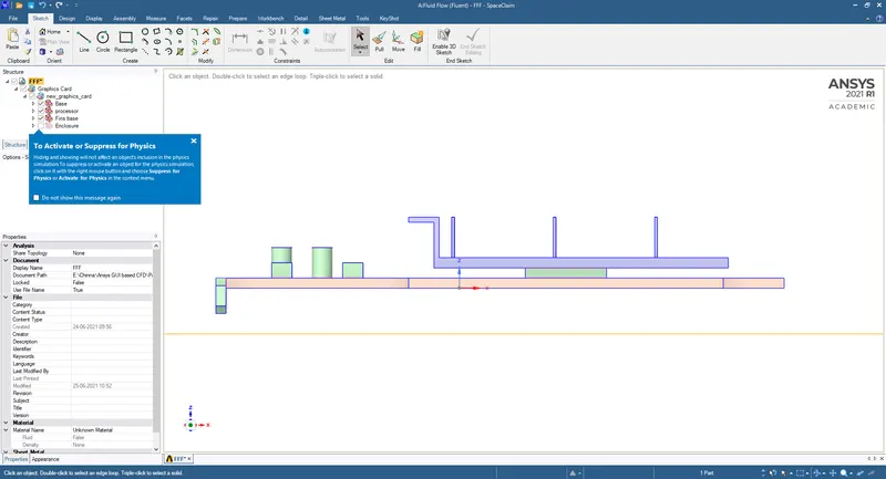
Now we enable the share topology option under FFF. This makes sure the mesh is continuous without overlapping.

We close SpaceClaim and update the geometry on workbench.

Meshing

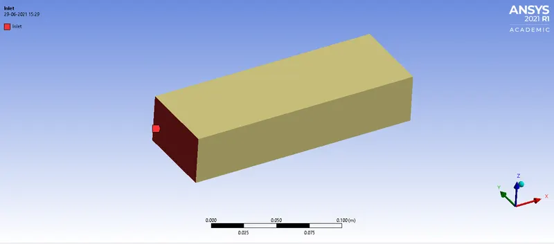
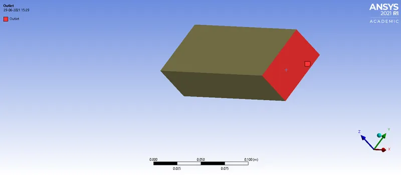
In the mesher, we first name the boundaries as follows

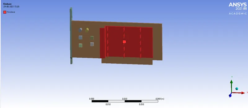
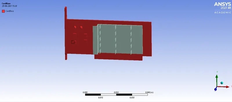
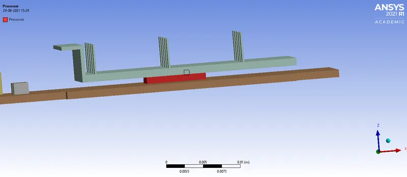
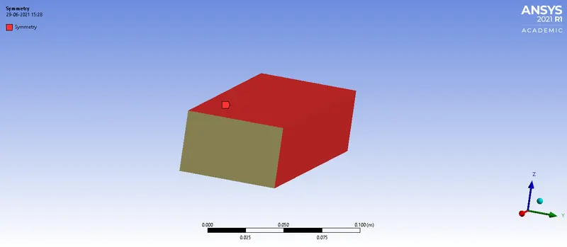
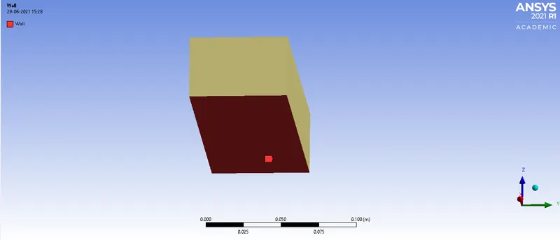
We use the body sizing options for finsbase, cardbase and the processor. We do this because we can reduce the number of cells and their size at these parts by reducing the cells in the enclosure.

Once everything is in place the mesh should look like this

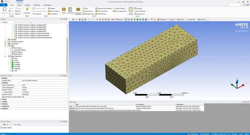
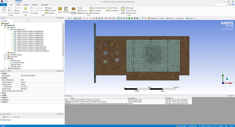
Now we export the mesh to the workbench and open the solver

Case Setup

In the solver, we choose a steady state, pressure based solver. We will also be solving for energy since temperature is involved.

The type of turbulence model used here is Standard K-`epsilon`model. Because K-`epsilon`models are most suitable for these kind of simulations.

Materials are

Finsbase - aluminium (Fluent database)

Fluid - air (Fluent database)

cardbase - copper (Fluent database)

Processor - silicon (modified)

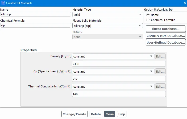
next, we define the zones at the appropriate regions such as

Cardbase > Solid

Finsbase > Solid

Enclosure > fluid

Processor > Solid

Here we define the source of heat as the processor this can be done in the edit processor option in the cellzone tab.

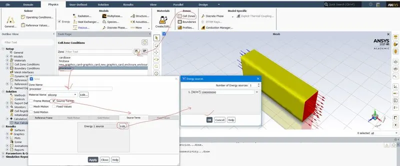
Here we need to define the internal heat generation. This can be given by the total power input by volume of the processor.

Most graphics cards of this size take an input of 70 Watts. The size of the processor is extracted from the spaceclaim.

The Initial and boundary conditions are as follows,

Inlet > Velocity inlet @ 5m/s, Inlet Fluid temperature is 300k.

we change this velocity to 1m/s and 3m/s and run two different cases so that we can compare these results to draw some meaning full conclusions

Outlet > Pressure Outlet @ 0pa Guage pressure, Backflow outlet temperature @ 300k

Now we initialise the solution using the hybrid initialisation method and set some monitors to capture the temperature contour. We also save this animation as we capture it.

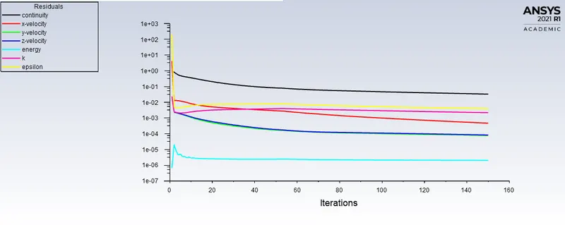
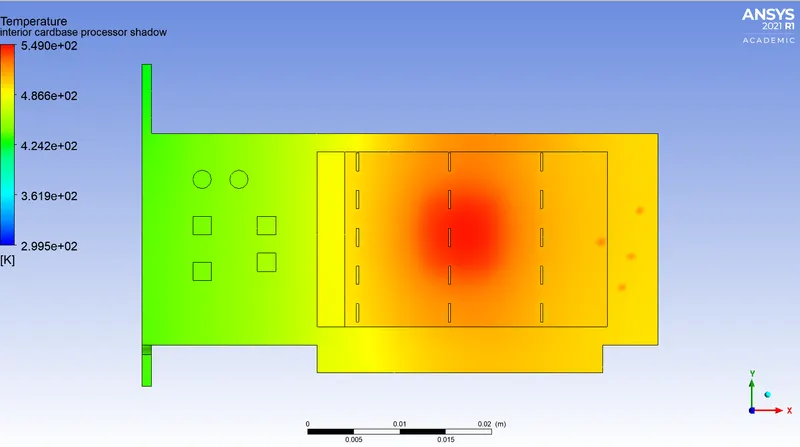
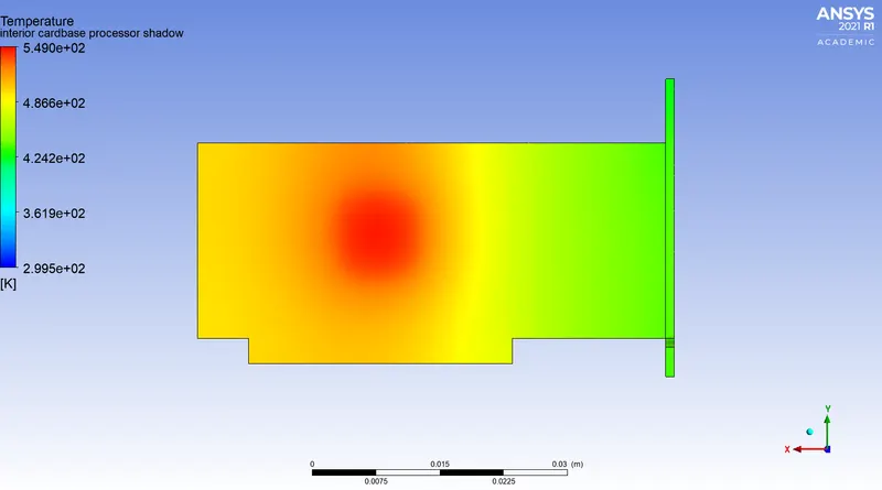
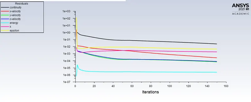
After everything is set we run the simulation for 150 iterations. Once the solution has converged we get the following results.

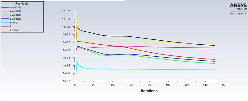
Residual plot

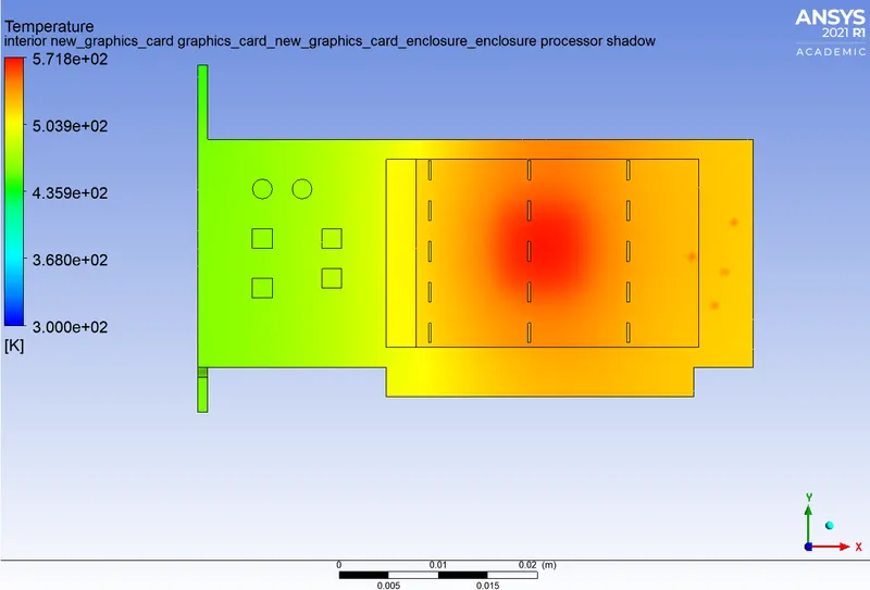
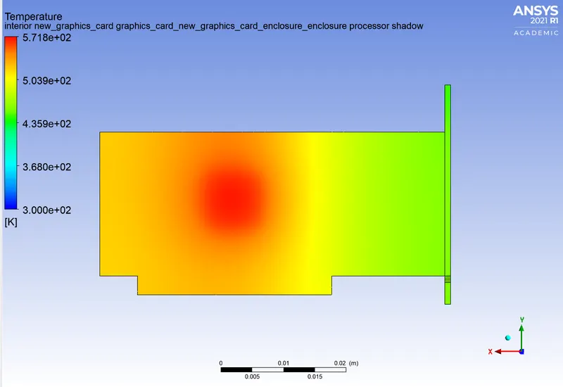
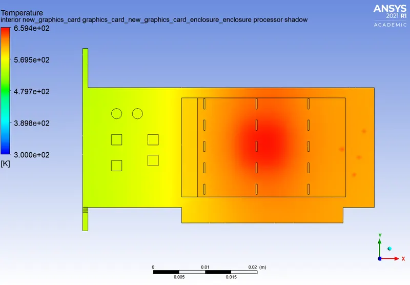
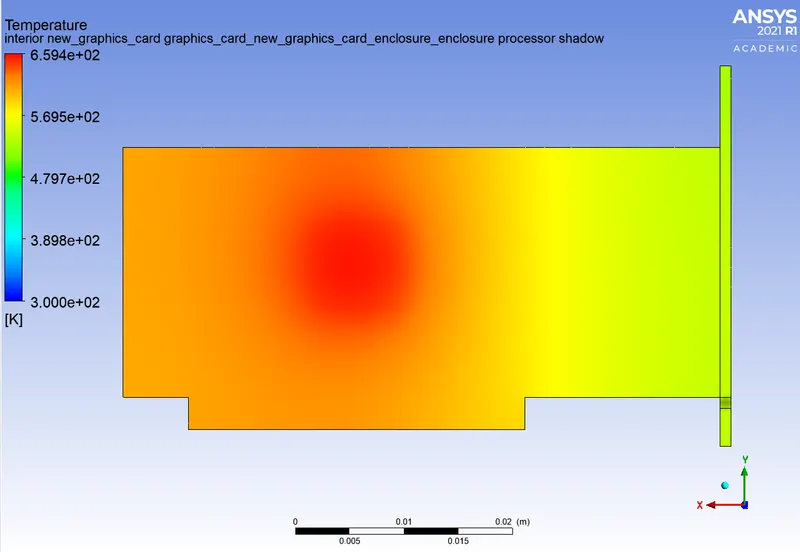
Temperature contour

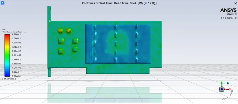
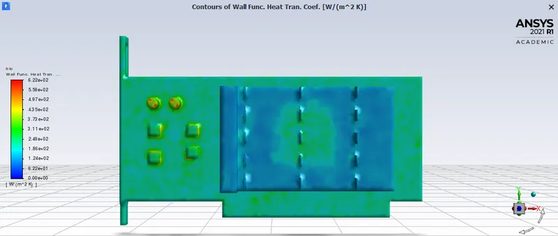
Wall heat transfer coefficient

For a velocity of 3m/s

Residual plot

Temperature contour

Wall heat transfer coefficient

For a velocity of 1m/s

Residual plot

Temperature contour

Wall heat transfer coefficient

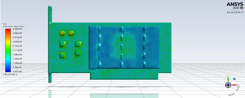
Maximum temperature on the processor at

1 m/s > 659.4 K

3 m/s > 571.8 K

5 m/s > 549.0 K

Maximum heat transfer coefficient on the processor is constant of 622 w/m^2-k.

CONCLUSION

The following conclusions have been made after observing the above plots and results

• The plots and animations show a constant contour after a some number iterations, Also the residuals lie below a particular value of 1e-1. from which we can say that the solution has converged.
• From the temperature plot we can say that the area of cardbase and the finbase around the processor is also getting heated. insufficient cooling in these areas may lead to damage of components.
• From the Heat transfer plot it can be seen that the cardbase has better heat transfer coefficient that the fins. This could be due to the material properties.
• From the above plots it can be seen that as the velocity of the air increases the maximum temperature on the graphics card decreases.
• The above point indicates that the as the fluid velocity increases the heat transfer through convection increases due to forced convection.